Wednesday, May 23, 2012
Wednesday, May 16, 2012
05-16-2012
7.2 Review
28. Pollen count distribution for Los Angeles in September is not normally distributed, with μ = 8.0, σ = 1.0, n = 64. Find P(x-bar > 9.0).
Is n ≥ 30 or the population is normally distributed? Population is not normally distributed, but n > 30, it's 64 so we can proceed with the problem and use the CLT.
The Central Limit Theorem says:
1) Shape: Approximately normal
2) Center: μ(subscripted x-bar) = μ, meaning the center for both the population and the sample is the same.
Thus μ = 8.0.
3) Spread: σ(subscripted x-bar) = σ/√ n (standard deviation divided by the square root of the sample size)
σ/√ n = 1.0 / √64 = 1/8 = 0.125
Now we draw a picture of a normal distributed centered at 8.0
Then add on what we're interested in: P(x-bar > 9.0).
So we move to the right and mark 9 then shade the area above 9.
Then use the z score formula to find the z score so we can find the probability.
9-8/0.125 = 8.0
A z-score of 8 is so large it's not listed on our table, meaning it's a very unusual observation. So we report the most extreme value we have, 3.49 = .9998
But since we wanted the area to the right, it's 1-0.9998 = .0002
0.02% probability of observing a pollen count greater than 9.0.
31. Boned trout prices are normally distributed, with μ = 3.10, σ = 0.30, n = 16. Find the sample mean price that is smaller than 90% of all sample means.
Is n ≥ 30 or the population is normally distributed? n < 30, but the population is normally distributed, so we can proceed with the problem and use the CLT.
The Central Limit Theorem says:
1) Shape: Normal
2) Center: μ(subscripted x-bar) = μ, meaning the center for both the population and the sample is the same.
Thus μ = 3.10.
3) Spread: σ(subscripted x-bar) = σ/√ n (standard deviation divided by the square root of the sample size)
σ/√ n = .30 / √16 = 0.30/4 = 0.075
Now we draw a picture of a normal distributed centered at 3.10
Then add on what we're interested in: "price that is smaller than 90% of all sample means." We are interested in the price where 90% of all observations are greater than it. Another way of saying this: we're interested in the 10th percentile.
P(x-bar < .1000).
So we move to the left of center and approximate the 10% mark and shade below it.
Now we're ready to use the z-score formula, unfortunately we're missing an observation but we have the percentage we're interested in! So we go to the Z-table and look for the Z value that corresponds to 0.1000 probability. We're looking at a Z-score of -1.28
So plugging into the z score formula:
x-3.1/0.075 = -1.28
x-3.10 = -0.096
x = 3.004
In conclusion, the 10th percentile for trout prices is $3.004 / lb.
51. College Board reports that the mean increase in SAT math scores of students who attend review courses is 18 points. Assume that the standard deviation is 12 points and that the change in score are not normally distributed. We are interested in the probability that the sample mean score increase is negative, indicating a loss of points after coaching. Suppose we take a sample of 40, and we are interested in P(x-bar<0), indicating a loss of points after coaching.
μ = 18
σ = 12
The Central Limit Theorem says:
1) Shape: Approximately normal (40>30)
2) Center: μ(subscripted x-bar) = μ, meaning the center for both the population and the sample is the same.
Thus μ = 18
3) Spread: σ(subscripted x-bar) = σ/√ n (standard deviation divided by the square root of the sample size)
σ/√ n = 12 / √40 = 12/2√10 = 1.897 = 1.90
Now we're ready to use the z-score formula, so plugging into the z score formula:
(0-18) / 1.897 = -9.49
However, the most extreme value on the z-table is -3.49. Finding this probability on the z-table: 0.0002
In conclusion, the probability that a person who received coaching would earn a 0 on the SAT is 0.02%
7.3 #44)
Shaq lead the league with a 58.4% goal percentage.
a) Find the minimum sample size that produces a sampling distribution of p-hat that is approximately normal
When dealing with proportions we have to make sure np ≥ 5 AND n(1-p) ≥ 5. This question is asking us to solve for n algebraically.
a1) n(.584)>5 (dividing both sides by .584)
n> 5/.584 (simplifying)
n> 8.56 (rounding up because you cannot have 8.56 goals)
n>9
a2) n(1-.584)>5
n(.416)>5 (dividing both sides by .416)
n > 5 / .416 (simplifying)
n > 12.02 (rounding up because you cannot having 12.02 goals)
n > 13
In conclusion, the minimum sample size required is 13 because that makes both equations true.
13(.584) > 5 and 13(.416)>5
b) Find μ(subscripted p-hat) and σ(subscripted p-hat) when n = 50.
The Central Limit Theorem says:
1) Shape: Approximately normal [np>5 and n(1-p)>5]
2) Center: μ(subscripted p-hat) = μ, meaning the center for both the population and the sample is the same. Thus μ = 58.4
3) Spread: σ(subscripted p-hat) = √ [p(1-p)/n] (square root of the proportion multiplied by 1 minus the proportion divided by sample size)
√ [.584(1-0.584)/50] = √ [.584(1-0.584)/50] = √ 0.2429/50 = √ .0049 = 0.0697
c)Find the probability that in a sample of 200 shots, Shaq would score more than 120 baskets.
120/200 = .6
Given this proportion we can use the z-score formula
(.6-.584) / .0697 Stop! You can't use that standard deviation it only works for a sample size of 50, we need to recalculate it!
√ [.584(1-0.584)/200] = .0349
Returning to our z-score formula...
(.6-.584) / .0349 = .4591 = .46
Taking .46 to the Z table we find a probability of .6772
However we are interested in the probability he would score MORE than 120 so we want the area to the right, you know what that means! 1-.6772 = 0.3228
Note: this answer varies from the book's, this is because they forgot to recalculate the standard deviation to account of the increased sample size.
8.3 #27)
Find the margin of error E for a 95% confidence interval
a) 5 successes in 10 trials.
5/10 = .5
so p = .5
The margin of error formula is: E = Z α/2 (√ [p-hat(1-(p-hat))/n])
Plugging in what we have
E = Z α/2 (√ [0.5(1-0.5)/10]
E = Z α/2 (0.1581)
For this Z α/2 value we need to look at our confidence interval table provided in table 8.1 on pg. 391, similar to table 8.7 on page 422. (might be a good idea to put those on your note card, just saying...)
So Z α/2 for 95% is 1.96
E = 1.96 (.1581)
E = .3099
8.2 Confidence Intervals for Means
Introducing the T-Distribution: Similar to the Z-Distribution, but has more variability (meaning the data is more spread out)
Remember: Degrees of Freedom = n-1
Confidence Interval for means = x-bar ± T α/2 (s / √n)
Notice that the standard deviation is similar to the one used for CLT means, but here we have s rather than σ. What does this mean? s is the standard deviation of our sample.
8.2 #6)
We are taking a random sample from a normal population with σ unknown. Find T α/2
a) Confidence level 95%, sample size 10
Degrees of freedom = n-1
Plugging in: 10 -1 = 9
Now we go to the t table and look at the 95% confidence level for a df of 9: 2.262
b) Confidence level 95%, sample size 15
Degrees of freedom = n-1
Plugging in: 15 -1 = 14
Now we go to the t table and look at the 95% confidence level for a df of 14: 2.145
c) Confidence level 95%, sample size 20
Degrees of freedom = n-1
Plugging in: 20 -1 = 19
Now we go to the t table and look at the 95% confidence level for a df of 19: 2.093
13. Confidence level 95%, sample size 25, sample mean 10, sample standard deviation 5.
CI: 95%, n = 25, μ = 10, s = 5.
a) T α/2
df = n-1, 25-1 = 24. Go to the T table find CI for 95% and df = 24, 2.064
b)Margin of Error (E) = T α/2(s/√n)
Plugging in what we know: 2.064 (5/√25) = 2.064 (1) = 2.064
c) Confidence interval for μ given the indicated confidence interval
Lower bound = μ - T α/2(s/√n)
10 - 2.064 = 7.936
Upper bound = μ + T α/2(s/√n)
10 + 2.936 = 12.064
28. Pollen count distribution for Los Angeles in September is not normally distributed, with μ = 8.0, σ = 1.0, n = 64. Find P(x-bar > 9.0).
Is n ≥ 30 or the population is normally distributed? Population is not normally distributed, but n > 30, it's 64 so we can proceed with the problem and use the CLT.
The Central Limit Theorem says:
1) Shape: Approximately normal
2) Center: μ(subscripted x-bar) = μ, meaning the center for both the population and the sample is the same.
Thus μ = 8.0.
3) Spread: σ(subscripted x-bar) = σ/√ n (standard deviation divided by the square root of the sample size)
σ/√ n = 1.0 / √64 = 1/8 = 0.125
Now we draw a picture of a normal distributed centered at 8.0
Then add on what we're interested in: P(x-bar > 9.0).
So we move to the right and mark 9 then shade the area above 9.
Then use the z score formula to find the z score so we can find the probability.
9-8/0.125 = 8.0
A z-score of 8 is so large it's not listed on our table, meaning it's a very unusual observation. So we report the most extreme value we have, 3.49 = .9998
But since we wanted the area to the right, it's 1-0.9998 = .0002
0.02% probability of observing a pollen count greater than 9.0.
31. Boned trout prices are normally distributed, with μ = 3.10, σ = 0.30, n = 16. Find the sample mean price that is smaller than 90% of all sample means.
Is n ≥ 30 or the population is normally distributed? n < 30, but the population is normally distributed, so we can proceed with the problem and use the CLT.
The Central Limit Theorem says:
1) Shape: Normal
2) Center: μ(subscripted x-bar) = μ, meaning the center for both the population and the sample is the same.
Thus μ = 3.10.
3) Spread: σ(subscripted x-bar) = σ/√ n (standard deviation divided by the square root of the sample size)
σ/√ n = .30 / √16 = 0.30/4 = 0.075
Now we draw a picture of a normal distributed centered at 3.10
Then add on what we're interested in: "price that is smaller than 90% of all sample means." We are interested in the price where 90% of all observations are greater than it. Another way of saying this: we're interested in the 10th percentile.
P(x-bar < .1000).
So we move to the left of center and approximate the 10% mark and shade below it.
Now we're ready to use the z-score formula, unfortunately we're missing an observation but we have the percentage we're interested in! So we go to the Z-table and look for the Z value that corresponds to 0.1000 probability. We're looking at a Z-score of -1.28
So plugging into the z score formula:
x-3.1/0.075 = -1.28
x-3.10 = -0.096
x = 3.004
In conclusion, the 10th percentile for trout prices is $3.004 / lb.
51. College Board reports that the mean increase in SAT math scores of students who attend review courses is 18 points. Assume that the standard deviation is 12 points and that the change in score are not normally distributed. We are interested in the probability that the sample mean score increase is negative, indicating a loss of points after coaching. Suppose we take a sample of 40, and we are interested in P(x-bar<0), indicating a loss of points after coaching.
μ = 18
σ = 12
The Central Limit Theorem says:
1) Shape: Approximately normal (40>30)
2) Center: μ(subscripted x-bar) = μ, meaning the center for both the population and the sample is the same.
Thus μ = 18
3) Spread: σ(subscripted x-bar) = σ/√ n (standard deviation divided by the square root of the sample size)
σ/√ n = 12 / √40 = 12/2√10 = 1.897 = 1.90
Now we're ready to use the z-score formula, so plugging into the z score formula:
(0-18) / 1.897 = -9.49
However, the most extreme value on the z-table is -3.49. Finding this probability on the z-table: 0.0002
In conclusion, the probability that a person who received coaching would earn a 0 on the SAT is 0.02%
7.3 #44)
Shaq lead the league with a 58.4% goal percentage.
a) Find the minimum sample size that produces a sampling distribution of p-hat that is approximately normal
When dealing with proportions we have to make sure np ≥ 5 AND n(1-p) ≥ 5. This question is asking us to solve for n algebraically.
a1) n(.584)>5 (dividing both sides by .584)
n> 5/.584 (simplifying)
n> 8.56 (rounding up because you cannot have 8.56 goals)
n>9
a2) n(1-.584)>5
n(.416)>5 (dividing both sides by .416)
n > 5 / .416 (simplifying)
n > 12.02 (rounding up because you cannot having 12.02 goals)
n > 13
In conclusion, the minimum sample size required is 13 because that makes both equations true.
13(.584) > 5 and 13(.416)>5
b) Find μ(subscripted p-hat) and σ(subscripted p-hat) when n = 50.
The Central Limit Theorem says:
1) Shape: Approximately normal [np>5 and n(1-p)>5]
2) Center: μ(subscripted p-hat) = μ, meaning the center for both the population and the sample is the same. Thus μ = 58.4
3) Spread: σ(subscripted p-hat) = √ [p(1-p)/n] (square root of the proportion multiplied by 1 minus the proportion divided by sample size)
√ [.584(1-0.584)/50] = √ [.584(1-0.584)/50] = √ 0.2429/50 = √ .0049 = 0.0697
c)Find the probability that in a sample of 200 shots, Shaq would score more than 120 baskets.
120/200 = .6
Given this proportion we can use the z-score formula
(.6-.584) / .0697 Stop! You can't use that standard deviation it only works for a sample size of 50, we need to recalculate it!
√ [.584(1-0.584)/200] = .0349
Returning to our z-score formula...
(.6-.584) / .0349 = .4591 = .46
Taking .46 to the Z table we find a probability of .6772
However we are interested in the probability he would score MORE than 120 so we want the area to the right, you know what that means! 1-.6772 = 0.3228
Note: this answer varies from the book's, this is because they forgot to recalculate the standard deviation to account of the increased sample size.
8.3 #27)
Find the margin of error E for a 95% confidence interval
a) 5 successes in 10 trials.
5/10 = .5
so p = .5
The margin of error formula is: E = Z α/2 (√ [p-hat(1-(p-hat))/n])
Plugging in what we have
E = Z α/2 (√ [0.5(1-0.5)/10]
E = Z α/2 (0.1581)
For this Z α/2 value we need to look at our confidence interval table provided in table 8.1 on pg. 391, similar to table 8.7 on page 422. (might be a good idea to put those on your note card, just saying...)
So Z α/2 for 95% is 1.96
E = 1.96 (.1581)
E = .3099
8.2 Confidence Intervals for Means
Introducing the T-Distribution: Similar to the Z-Distribution, but has more variability (meaning the data is more spread out)
 |
| Notice: Due to the extra variability there is more info at the extremes. |
Remember: Degrees of Freedom = n-1
Confidence Interval for means = x-bar ± T α/2 (s / √n)
Notice that the standard deviation is similar to the one used for CLT means, but here we have s rather than σ. What does this mean? s is the standard deviation of our sample.
8.2 #6)
We are taking a random sample from a normal population with σ unknown. Find T α/2
a) Confidence level 95%, sample size 10
Degrees of freedom = n-1
Plugging in: 10 -1 = 9
Now we go to the t table and look at the 95% confidence level for a df of 9: 2.262
b) Confidence level 95%, sample size 15
Degrees of freedom = n-1
Plugging in: 15 -1 = 14
Now we go to the t table and look at the 95% confidence level for a df of 14: 2.145
c) Confidence level 95%, sample size 20
Degrees of freedom = n-1
Plugging in: 20 -1 = 19
Now we go to the t table and look at the 95% confidence level for a df of 19: 2.093
13. Confidence level 95%, sample size 25, sample mean 10, sample standard deviation 5.
CI: 95%, n = 25, μ = 10, s = 5.
a) T α/2
df = n-1, 25-1 = 24. Go to the T table find CI for 95% and df = 24, 2.064
b)Margin of Error (E) = T α/2(s/√n)
Plugging in what we know: 2.064 (5/√25) = 2.064 (1) = 2.064
c) Confidence interval for μ given the indicated confidence interval
Lower bound = μ - T α/2(s/√n)
10 - 2.064 = 7.936
Upper bound = μ + T α/2(s/√n)
10 + 2.936 = 12.064
Monday, May 14, 2012
05-14-2012
Central Limit Theorem for Proportions (p-hat)
The Central Limit Theorem maintains:
1) Shape: Is normal or approximately normal
2) Center: μ(subscripted p-hat) = P, meaning the center for both the population and the sample is the same.
3) Spread: σ(subscripted p-hat) = √[(p(1-p))/n]
Note: We can only use the CLT for proportion when np ≥ 5 AND n(1-p) ≥ 5
Confidence Intervals - How certain do you want to be that you caught the population value?
Table derived from table 8.1 on pg. 391, similar to table 8.7 on page 422.
We observed a bag with a proportion of .48 orange candies, but we don't know that the factory desires a 0.40 proportion for orange candies. Suppose we want to be 95% confident that our observation of 0.48 was within the factory specification.
To find our confidence intervals we'll use the following formula which can be found on p.391
Lower bound = x-bar - Z α/2(σ/√n)
Upper bound = x-bar + Z α/2(σ/√n)
So plugging in to find out lower bound...
Lower bound = 0.48 - 1.96(0.0980) = 0.2879
Upper bound = 0.48 + 1.96(0.0980) = 0.6721
In conclusion, we're 95% that the true proportion of orange candies in a given bag of Reese's Pieces will fall between 0.2879 and 0.6721.
What if we wanted to be 99% confident?
Simply changing the Z α/2 to reflect our desired confidence interval:
Lower bound = 0.48 - 2.576(0.0980) = 0.2276
Upper bound = 0.48 + 2.576(0.0980) = 0.7324
In conclusion, we're 99% that the true proportion of orange candies in a given bag of Reese's Pieces will fall between 0.2276 and 0.7324.
In all reality we'll never know the true proportion of any given observation, so how do we adjust for this? We continue using the CLT for proportion but replace every instance of P (population proportion) with p-hat (our sample proportion). Use p-hat instead of P
Given
n = 25
p-hat = 0.48
standard deviation = √ [(P(1-P))/n]
But wait, we don't have P, what ever will we do? Use p-hat!
so plugging in: √[(0.48(1-0.48))/25] = 0.0999
Predicting a 95% confidence interval for this data...
Lower bound = 0.48 - 1.96 (.0999) = 0.2842
Upper bound = 0.48 + 1.96(.0999) = 0.6758
Margin of error = Z α/2(σp-hat)
Please note that the margin of error is exactly the same as portion of the confidence interval formula that lies to the right of the operation symbol (±).
Hypothesis Testing - Think of this as "looking for how much evidence we have against the null hypothesis" or "Using Statistics to answer a question"
Suppose that a recent poll reported that 49% of the United States is pro-choice, however you think it's higher.
You need to do a few things:
1) Form a null hypothesis (H0) which assumes the original value is true (status quo).
2) Offer an alternate hypothesis (HA) in which you make your claim. HA: P ≠ P0, P > P0, or P < P0 . In this example we are assuming P > P0.
3) Get sample and find a test statistic (Use the Z Score formula)
4) Go to the chart and find the P-Value for your Z Score of interest.
5) Conclusion
The Central Limit Theorem maintains:
1) Shape: Is normal or approximately normal
2) Center: μ(subscripted p-hat) = P, meaning the center for both the population and the sample is the same.
3) Spread: σ(subscripted p-hat) = √[(p(1-p))/n]
Note: We can only use the CLT for proportion when np ≥ 5 AND n(1-p) ≥ 5
Confidence Intervals - How certain do you want to be that you caught the population value?
Table derived from table 8.1 on pg. 391, similar to table 8.7 on page 422.
| Confidence Level (1 - α)100% | α | α/2 | Z α/2 |
|---|---|---|---|
| 100(1-0.15)% = 85% | 0.15 | 0.075 | 1.44 |
| 100(1-0.10)% = 90% | 0.10 | 0.05 | 1.645 |
| 100(1-0.05)% = 95% | .05 | 0.025 | 1.96 |
| 100(1-0.01)% = 99% | .01 | 0.005 | 2.576 |
We observed a bag with a proportion of .48 orange candies, but we don't know that the factory desires a 0.40 proportion for orange candies. Suppose we want to be 95% confident that our observation of 0.48 was within the factory specification.
To find our confidence intervals we'll use the following formula which can be found on p.391
Lower bound = x-bar - Z α/2(σ/√n)
Upper bound = x-bar + Z α/2(σ/√n)
So plugging in to find out lower bound...
Lower bound = 0.48 - 1.96(0.0980) = 0.2879
Upper bound = 0.48 + 1.96(0.0980) = 0.6721
In conclusion, we're 95% that the true proportion of orange candies in a given bag of Reese's Pieces will fall between 0.2879 and 0.6721.
What if we wanted to be 99% confident?
Simply changing the Z α/2 to reflect our desired confidence interval:
Lower bound = 0.48 - 2.576(0.0980) = 0.2276
Upper bound = 0.48 + 2.576(0.0980) = 0.7324
In conclusion, we're 99% that the true proportion of orange candies in a given bag of Reese's Pieces will fall between 0.2276 and 0.7324.
In all reality we'll never know the true proportion of any given observation, so how do we adjust for this? We continue using the CLT for proportion but replace every instance of P (population proportion) with p-hat (our sample proportion). Use p-hat instead of P
Given
n = 25
p-hat = 0.48
standard deviation = √ [(P(1-P))/n]
But wait, we don't have P, what ever will we do? Use p-hat!
so plugging in: √[(0.48(1-0.48))/25] = 0.0999
Predicting a 95% confidence interval for this data...
Lower bound = 0.48 - 1.96 (.0999) = 0.2842
Upper bound = 0.48 + 1.96(.0999) = 0.6758
Margin of error = Z α/2(σp-hat)
Please note that the margin of error is exactly the same as portion of the confidence interval formula that lies to the right of the operation symbol (±).
Hypothesis Testing - Think of this as "looking for how much evidence we have against the null hypothesis" or "Using Statistics to answer a question"
Suppose that a recent poll reported that 49% of the United States is pro-choice, however you think it's higher.
You need to do a few things:
1) Form a null hypothesis (H0) which assumes the original value is true (status quo).
2) Offer an alternate hypothesis (HA) in which you make your claim. HA: P ≠ P0, P > P0, or P < P0 . In this example we are assuming P > P0.
3) Get sample and find a test statistic (Use the Z Score formula)
4) Go to the chart and find the P-Value for your Z Score of interest.
- P(Z > z) for P > P0
- P(Z < z) for P < P0
- 2P(Z<z) = P ≠ P0
5) Conclusion
Wednesday, May 9, 2012
05-09-2012
Central Limit Theorem (CLT) for Means (x-bar) - Allows us to figure out how samples of varying sizes behave in the long run.
The Central Limit Theorem states that:
1) Shape: Is normal or approximately normal
2) Center: μ(subscripted x-bar) = μ, meaning the center for both the population and the sample is the same.
3) Spread: σ(subscripted x-bar) = σ/√ n (standard deviation divided by the square root of the sample size)
Note: We can only use the CLT when n ≥ 30 OR the population is normally distributed
Example 7.12 (p. 357)
μ = 12, 485
σ = 21,973
n = 10
Notice that the standard deviation is enormous looking at the provided histogram we observe that our distribution is right skewed. Thus, the distribution is NOT normally distributed. If we use the CLT to proceed we will get inaccurate data. Therefore we do not continue because we do not have enough information.
Now let's suppose our sample size was 36 as opposed to 10.
Now that n ≥ 30, we can use the CLT.
So using what we know about the CLT we can conclude three things.
1) Shape. Shape will be approximately normal
2) Center. Centered at μ (12, 485)
3) Spread.σ/√ n. Plugging in 21973/√ 36 = 21973/6 = 3662.17
Suppose we are interested in the probability that the mean is greater than 17,000.
p(x-bar > 17,000)
In order to solve this problem, we are going to use the Z-score formula
 |
| z = (observed - expected) / standard deviation |
So for this problem:
(17000-12485) / 3662.17 = 1.23
Going to the Z-table with this value of 1.23 we find a value of 0.8907.
However the question posed was the probability of finding a sample mean greater than 17,000 so we need to do 1-0.8907 to find the area to the right. Subtracting we find the probability of finding a sample mean higher than 17,000 to be 0.1093. Interpretation: 10.93% chance that a random sample size of 36 cities will give you greater than 17,000 small businesses.
Central Limit Theorem for Proportions (p-hat)
The Central Limit Theorem maintains:
1) Shape: Is normal or approximately normal
2) Center: μ(subscripted p-hat) = P, meaning the center for both the population and the sample is the same.
3) Spread: σ(subscripted p-hat) = √[(p(1-p))/n]
Note: We can only use the CLT for proportion when np ≥ 5 AND n(1-p) ≥ 5
In class example with Reese's Pieces applet.
We are interested in the proportion of candies that are orange.
Setting π = 0.40 (makes the simulation machine produce 40% orange candies)
n = 25
Then draw a sample, Brandon got 0.36.
Applying what the Central Limit Theorem tells us about sampling variability.
1) Shape: Is normal or approximately normal
2) Center: μ(subscripted p-hat) = 0.4
3) Spread: σ(subscripted p-hat) = √[(0.4(1-0.4))/25] = .0979 = .0980
Checking to see if it meets the prerequisite criteria: 25(0.4) = 10. 10 > 5, so we're good there.
25(1-0.4) = 15, 15>5. Both criteria have been met.
What's the probability of observing a bag of Reese's pieces with 24% orange candies?
Z score time!
( 0.24 - 0.4 ) / 0.098 = -1.63
Finding -1.63 on the z table, we find that the probability is .0576.
Interpretation: 5.76% chance of finding a package with 24% or fewer orange candies.
What's the probability of observing a bag of Reese's Pieces with 60% or greater orange candies?
( 0.6 - 0.4 ) / 0.098 = 2.04
Find 2.04 on the Z table, we find the probability to be 0.9793. However, that .9793 refers to the area to the left, we're interested in the area to the right, so we do 1-0.9793 and find the the probability to be .0207.
Interpretation: 2.07% chance of finding a packaged with 60% or greater orange candies in any given package of Reese's Pieces.
If the class continues to take increasingly larger samples we tighten up the variability and come closer to our intended proportion of 0.40. Observe the trend in the table below:
| Sample Size (n) | Class Low | Class High |
|---|---|---|
| 25 | .24 | .60 |
| 50 | .22 | .50 |
| 75 | .29 | .53 |
| 100 | .30 | .52 |
| 500 | .36 | .43 |
The larger the sample size the closer the values are to our intended 0.40.
In order to cut the standard deviation in half you need to quadruple the sample size.
Monday, May 7, 2012
05-07-2012
Sampling Distribution - Pattern of Variability for Samples
Quantitative - Involves numbers, denoted by x-bar and used to predict μ (population parameters)
Qualitative (categorical) - Involves objects other than numbers (e.g. hair color or gender), denoted by p-hat and used to predict P (proportion parameters).
In Class Skittles Exercise
Each student was given a fun size package of skittles and asked to record:
1) Total number of skittles
2) Number of purple and red skittles (combined)
3) Proportion of skittles per package that are red and purple (combined)
The total is quantitative (number)
The proportion is categorical because it's a color reported.
Sample size = 36 students in the class
Normally distributed - Average number of skittles per package 16
X-bar (mean): 15.125
Standard deviation: 1.328
If you are asked to report your mean? Just report the number of candies present in your bag.
Although better estimates come from taking larger sample sizes or taking more samples.
Central Limit Theorem (CLT) for Means (x-bar) - Allows us to figure out how samples of varying sizes behave in the long run.
The Central Limit Theorem states that:
1) Shape: Is normal or approximately normal
2) Center: μ(subscripted x-bar) = μ, meaning the center for both the population and the sample is the same.
3) Spread: σ(subscripted x-bar) = σ/√ n (standard deviation divided by the square root of the sample size)
Note: We can only use the CLT when n ≥ 30 or the population is normally distributed
Saturday, May 5, 2012
05-03-2012
Walk through on how to solve the types of Problems encountered in 6.5 [video]
7.1 Sampling Error
Sampling error - Absolute value of the difference between statistic and parameter.
Mean: | x-bar - μ |
Standard deviation: | s - σ |
Proportion: | p-bar - P |
μ - Population (Parameter) mean
x-bar - Sample (Statistic) mean or "Point estimate"
7.1 Sampling Error
Sampling error - Absolute value of the difference between statistic and parameter.
Mean: | x-bar - μ |
Standard deviation: | s - σ |
Proportion: | p-bar - P |
μ - Population (Parameter) mean
x-bar - Sample (Statistic) mean or "Point estimate"
Monday, April 23, 2012
04-23-2012
 |
| Remember me? |
- The area under the curve is always equal to one (1.0), because the total probability for any event is 1.0 (As you may recall the probability of 1 means that the event always happens or has a 100% probability - which is our maximum)
- The distribution is always centered around the mean (µ), which has a standard deviation of 0. 50% of the data lies above the mean and 50% of the data lies below the mean.
- To find Z scores:

Z Table (pdf) - Gives you area under the curve for the specific standard deviation you are interested in.
Normal distribution (java applet) - Helps you visualize what you are trying to find
What is the area to the left of Z-score value 0.57?
First we find the 0.5 row under the Z column on the table, then move across that row to find 0.07. This will give us the area under the curve at 0.57 which is: 0.7157
p(Z<0.57) = 0.7157
Suppose we want to know the area to the right of the Z-score 0.57, how would we do that given that the Z-Table only provides us with area to the LEFT of the Z score? Well we use our knowledge that the entire curve accounts for a total probability of 1. If we remove the section to the left (which we can find easily from the Z-table) we will be left with the area to the right!
p(Z>0.57) = 1 - 0.7157
p(Z>0.57) = 0.2843
Alternatively, the area to the right of the positive value is same as the area to the left of negative value due to the symmetric nature of the distribution.
p(Z>0.57) = p(Z<-0.57) = 0.2843
Remember the Empirical Rule? You know, one standard deviation being 68%, two standard deviations being 95% and three standard deviations being 99.7%? Well let's see how accurate that rule of thumb is.
So what is the probability that Z is greater than negative one standard deviation and less than one standard deviation? p(-1 < Z < 1) ?
To find the area between two points it's best to approach it as two separate problems, so let's find the highest value first.
Let's draw a picture of what we're trying to find so we can visualize the problem, this java applet should help you on your way.
Looking at the Z table, what's the probability that Z is less than positive one? p (Z < 1.00) = 0.8413
Looking at the Z table, what's the probability that Z is less than negative one? p(Z < -1.00) = 0.1587
Since we are interested in the area between -1 and 1, we don't really want the area to the left of -1 as we have found, so we can just subtract it from the area to the left of positive 1 and we will have our answer.
0.8413 - 0.1587 = .6826
p(-1 < Z < 1) = .6826, or 68.26% of the data lies between 1 standard deviation
Pretty close to the Empirical Rule's estimate of 68% of the data falling within 1 standard deviation.
p(-2 < Z < 2) ?
p(Z<2.00) = 0.9772
p(Z<-2.00) = 0.0228
p(-2 < Z < 2) = 0.9772 - 0.0228
p(-2 < Z < 2) = 0.9544
Again, pretty to the Empirical Rule's estimate of 95%
p(-3 < Z < 3) ?
p(Z<3.00) = 0.9987
p(Z<-3.00) = 0.0013
p(-3 < Z < 3) = 0.9987 - 0.0013
p(-3 < Z < 3) = 0.9974
Also close to the Empirical Rule's estimate of 99.7%
But what if we wanted to know what Z scores correspond with exactly 68%?
Well if we know the entire area under the curve is 100% or 1.0 and we want to capture the middle 68%
1-0.68 = 0.32 so there will be 32% of the data unaccounted for, but this is not at one end, it's distributed evenly at both tails because the distribution is symmetric. So 0.32/2 = 0.16
1-0.16 = 0.8400
Now we go to the Z-Table and look for the value closest to 0.8400, after some searching we find the values 0.8365 (located at 0.98), 0.8389 (located at 0.99), and 0.8413 (located at 1.0). Unfortunately 0.8413 is greater than 0.8400 so we will go with the next highest value 0.8389. So if we're interested in the middle 68% we're looking at p( -0.99 < Z < 0.99)
Wednesday, April 18, 2012
04-16-2012
Binomial Distribution
1) 2 possible outcomes
2) Fixed number of trials
3) Independent events
4) Probability is constant
The Binomial Formula
 p = Probability
n = number of trials
x = number of successes
"At most" means "less than or equal to". Ex: If I wanted at most 5, I am interested in the probabilities between 0 and 5. [p(0)+p(1)+p(2)+p(3)+p(4)+p(5)]
"At least" means "greater than or equal to". Ex: If I wanted at least 5 in a sample of ten, I am interested in the probabilities between 5 and 10. [p(5)+p(6)+p(7)+p(8)+p(9)+p(10)]
6.2 # 13-18, the experiment is to toss a fair coin three times. Use the binomial formula to find the indicated probabilities.
13. No heads were observed.
p = 0.50 , n = 3, x = 0.
p(0) = 3C0 (0.5)0 (1-.0.5)(3-0)
p(0) = (1) (1) (0.125)
p(0) = 0.125
14. One head was observed.
p = 0.50 , n = 3, x = 1.
p(1) = 3C1 (0.5)1 (1-.0.5)(3-1)
p(1) = (3) (0.5) (0.25)
p(1) = 0.375
15. Two heads were observed
p = 0.50 , n = 3, x = 2.
p(2) = 3C2 (0.5)2 (1-.0.5)(3-2)
p(2) = (3) (0.25) (0.5)
p(2) = 0.375
16. Three heads were observed.
p = 0.50 , n = 3, x = 3.
p(3) = 3C3 (0.5)3 (1-.0.5)(3-3)
p(3) = (1) (0.125) (1)
p(3) = 0.125
17. At most two heads were observed.
"At most" refers to a combined probability, in this case it's "less than or equal to" two heads. So we are interested in the cumulative probability from 0 to 2, which we already found in the previous problems so...
p(0) + p(1) + p(2) = ?
0.125 + 0.375 + 0.375 = 0.875
18. More than two heads were observed
"More than" refers to a combined probability, in this case it's "greater than" two heads. So we are interested in the probabilities greater than 3, however for this problem set there is only one such probability that matches this...
p(3) = 0.125
22. Probability that at least 3 of the next 4 dentists surveyed will recommend sugarless gum. Assume the recommendation is given 95% of the time.
"At least" refers to a combined probability, in this case we're interested in a minimum of 3 successes. So we need to find probability of observing a 3 and the probability of observing a 4.
p(3) = 4C3 (0.95)3 (1-0.95)(4-3)
p(3) = (4) (0.857375) (.05)
p(3) = 0.1715
p(4) = 4C4 (0.95)4 (1-0.95)(4-4)
p(4) = (1) (0.81450625) (1)
p(4) = 0.8145
p(3+4) = 0.8145 + 0.1715
p(3+4) = 0.8145 + 0.1715
p(3+4) = 0.9860
If you are unclear on any of this, please watch this video.
1) 2 possible outcomes
2) Fixed number of trials
3) Independent events
4) Probability is constant
The Binomial Formula
n = number of trials
x = number of successes
"At most" means "less than or equal to". Ex: If I wanted at most 5, I am interested in the probabilities between 0 and 5. [p(0)+p(1)+p(2)+p(3)+p(4)+p(5)]
"At least" means "greater than or equal to". Ex: If I wanted at least 5 in a sample of ten, I am interested in the probabilities between 5 and 10. [p(5)+p(6)+p(7)+p(8)+p(9)+p(10)]
6.2 # 13-18, the experiment is to toss a fair coin three times. Use the binomial formula to find the indicated probabilities.
13. No heads were observed.
p = 0.50 , n = 3, x = 0.
p(0) = 3C0 (0.5)0 (1-.0.5)(3-0)
p(0) = (1) (1) (0.125)
p(0) = 0.125
14. One head was observed.
p = 0.50 , n = 3, x = 1.
p(1) = 3C1 (0.5)1 (1-.0.5)(3-1)
p(1) = (3) (0.5) (0.25)
p(1) = 0.375
15. Two heads were observed
p = 0.50 , n = 3, x = 2.
p(2) = 3C2 (0.5)2 (1-.0.5)(3-2)
p(2) = (3) (0.25) (0.5)
p(2) = 0.375
16. Three heads were observed.
p = 0.50 , n = 3, x = 3.
p(3) = 3C3 (0.5)3 (1-.0.5)(3-3)
p(3) = (1) (0.125) (1)
p(3) = 0.125
17. At most two heads were observed.
"At most" refers to a combined probability, in this case it's "less than or equal to" two heads. So we are interested in the cumulative probability from 0 to 2, which we already found in the previous problems so...
p(0) + p(1) + p(2) = ?
0.125 + 0.375 + 0.375 = 0.875
18. More than two heads were observed
"More than" refers to a combined probability, in this case it's "greater than" two heads. So we are interested in the probabilities greater than 3, however for this problem set there is only one such probability that matches this...
p(3) = 0.125
22. Probability that at least 3 of the next 4 dentists surveyed will recommend sugarless gum. Assume the recommendation is given 95% of the time.
"At least" refers to a combined probability, in this case we're interested in a minimum of 3 successes. So we need to find probability of observing a 3 and the probability of observing a 4.
p(3) = 4C3 (0.95)3 (1-0.95)(4-3)
p(3) = (4) (0.857375) (.05)
p(3) = 0.1715
p(4) = 4C4 (0.95)4 (1-0.95)(4-4)
p(4) = (1) (0.81450625) (1)
p(4) = 0.8145
p(3+4) = 0.8145 + 0.1715
p(3+4) = 0.8145 + 0.1715
p(3+4) = 0.9860
If you are unclear on any of this, please watch this video.
Wednesday, April 11, 2012
04-11-2012
Section 5.3, page 234
Sampling with replacement - Each trial is an independent event. (e.g. pulling names from a hat and returning the names to the hat after they've been pulled)
Sampling without replacement - Each trial is a dependent event, odds of an event happening increase with each trial (e.g pulling a name from a hat, and don't replace them, if you continue to pull names your name will eventually come up- thus your odds increase with each trial).
ELISA test of HIV example
The ELISA test reports a positive result 99.6% if blood has HIV, therefore it reports a false negative (meaning the test says you don't have HIV, but you do) 0.4% of the time (1-.996 = .004)
If blood has no HIV the test reports a negative result 98% of the time, conversely the false positive (meaning the test says you have HIV, but you don't) rate is 2% (1-.98 = .02).
If the prevalence of HIV is 0.5% and we collect blood samples from 100,000 randomly selected people.
How many people will have HIV?
Well if 0.5% of the population have HIV and we have 100,000 people, we simply multiply the population by the percentage: (0.005)*(100000) = 500.
500 people will have HIV
How many people do not have HIV?
100000 - 500 = 99500.
99500 will not have HIV
How many of the 500 HIV positive people will the test detect?
The test accurately reports positive 99.6% of the time if the blood has HIV, so (0.996)* (500) = 498
498 HIV positive people will be detected by the test
How many of the 500 HIV positive people will the test miss?
The test erroneously reports negative (false negative) 0.4% of the time if the blood has HIV, so (0.004) * (500) = 2
Alternatively, you could acknowledge that the false negative is the compliment of the positively detected group, so 500-498 = 2.
2 HIV positive people will be erroneously reported as HIV negative (missed by the test).
How many of the 99500 HIV negative people will the test detect?
The test accurately reports a negative result 98% of the time, so (0.98) * (99500) = 97510
97510 HIV negative people will be detected by the test
How many of the 99500 HIV negative people will the test miss?
The test erroneously reports positive (false positive) 2% of the time if the blood lacks HIV, so (0.02)*(99500) = 1990
Alternatively, you could acknowledge that the false positive is the compliment of the negatively detected group, so 99500-97510 = 1990
1990 HIV negative people will be erroneously reported as HIV positive (missed by the test).
Using this data to create a cross-tabulation table...
Proportion of people that are actually HIV positive given ELISA reported negative?
p(HIV+ | ELISA-) = 2 / 97512
p(HIV+ | ELISA-) = 0.00002051
0.002051% of the time ELISA will report negative when the sample is HIV positive
Proportion of people that are HIV positive given ELISA reported positive?
p(HIV+ | ELISA+) = 498 / 2488
p(HIV+ | ELISA+) = 0.200160772
20% of the time ELISA will report positive when the sample HIV positive
Proportion of people that are HIV negative given ELISA reported positive?
p(HIV- | ELISA+) = 1990 / 2488
p(HIV- | ELISA+) = 0.799839228
Nearly 80% of the time ELISA will report positive when sample HIV negative
Why would the ELISA be designed to report HIV positive when the sample is actually HIV negative more frequently than report HIV negative when the sample truly is HIV positive (false negative)?
A person who receives a false negative from ELISA could potentially spread the infection further given the epidemic nature of the illness. Thus, ELISA was designed in order to keep the false negative rate as low as possible.
6.1)
Discrete Random Variable - Specific number of probable outcomes. If you chose from the class - 40 possible outcomes.
Continuous Random Variable - If class ran a mile - Infinite number of possible outcomes.
If you would like to augment your knowledge of this subject, please watch this video.
6.2)
Binomial Distribution or Binomial "pattern of variability"
How do you determine if it's a Binomial Distribution?
Is flipping a coin three times for a heads a binomial distribution?
Suppose you wanted to grow your happy hypothetical family from 4 children to 10 children. What happens to the probability of having a female?
Calc> Random Data> Binomial Distribution> 1000 rows (trials), storing in C2, 10 trials, probability of event (.51)

Resulting data is stored in C2>

Stat> Tables> Tally Individual Variables> Select C2, include "Counts" and "Percents"> Select OK>

Interpreting results:
p(0 females) = 0%
p(1 females) = 0.7%
p(2 female) = 3.6%
p(3 females) = 10.2%
p(4 females) = 17.6%
p(5 females) = 26.9%
p(6 females) = 22.3%
p(7 females) = 12.8%
p(8 females) = 5.3%
p(9 females) = 0.6%
p(10 females) = 0%
What have we learned? The more trials (children) you have, the probability decreases. If you wanted the best odds of having a child of each gender you're best off stopping at 2 children, continuing to have kids will not increase the odds!
Sampling with replacement - Each trial is an independent event. (e.g. pulling names from a hat and returning the names to the hat after they've been pulled)
Sampling without replacement - Each trial is a dependent event, odds of an event happening increase with each trial (e.g pulling a name from a hat, and don't replace them, if you continue to pull names your name will eventually come up- thus your odds increase with each trial).
ELISA test of HIV example
The ELISA test reports a positive result 99.6% if blood has HIV, therefore it reports a false negative (meaning the test says you don't have HIV, but you do) 0.4% of the time (1-.996 = .004)
If blood has no HIV the test reports a negative result 98% of the time, conversely the false positive (meaning the test says you have HIV, but you don't) rate is 2% (1-.98 = .02).
If the prevalence of HIV is 0.5% and we collect blood samples from 100,000 randomly selected people.
How many people will have HIV?
Well if 0.5% of the population have HIV and we have 100,000 people, we simply multiply the population by the percentage: (0.005)*(100000) = 500.
500 people will have HIV
How many people do not have HIV?
100000 - 500 = 99500.
99500 will not have HIV
| Population | |
|---|---|
| HIV Positive |
500
|
| HIV Negative |
99500
|
How many of the 500 HIV positive people will the test detect?
The test accurately reports positive 99.6% of the time if the blood has HIV, so (0.996)* (500) = 498
498 HIV positive people will be detected by the test
How many of the 500 HIV positive people will the test miss?
The test erroneously reports negative (false negative) 0.4% of the time if the blood has HIV, so (0.004) * (500) = 2
Alternatively, you could acknowledge that the false negative is the compliment of the positively detected group, so 500-498 = 2.
2 HIV positive people will be erroneously reported as HIV negative (missed by the test).
How many of the 99500 HIV negative people will the test detect?
The test accurately reports a negative result 98% of the time, so (0.98) * (99500) = 97510
97510 HIV negative people will be detected by the test
How many of the 99500 HIV negative people will the test miss?
The test erroneously reports positive (false positive) 2% of the time if the blood lacks HIV, so (0.02)*(99500) = 1990
Alternatively, you could acknowledge that the false positive is the compliment of the negatively detected group, so 99500-97510 = 1990
1990 HIV negative people will be erroneously reported as HIV positive (missed by the test).
Using this data to create a cross-tabulation table...
| Actually Positive (+) | Actually Negative (-) | Total | |
|---|---|---|---|
| Test Positive (+) |
498
|
1990
|
2488 |
| Test Negative (-) |
2
|
97510
|
97512 |
| Total |
500
|
99500
|
100000 |
Proportion of people that are actually HIV positive given ELISA reported negative?
p(HIV+ | ELISA-) = 2 / 97512
p(HIV+ | ELISA-) = 0.00002051
0.002051% of the time ELISA will report negative when the sample is HIV positive
Proportion of people that are HIV positive given ELISA reported positive?
p(HIV+ | ELISA+) = 498 / 2488
p(HIV+ | ELISA+) = 0.200160772
20% of the time ELISA will report positive when the sample HIV positive
Proportion of people that are HIV negative given ELISA reported positive?
p(HIV- | ELISA+) = 1990 / 2488
p(HIV- | ELISA+) = 0.799839228
Nearly 80% of the time ELISA will report positive when sample HIV negative
Why would the ELISA be designed to report HIV positive when the sample is actually HIV negative more frequently than report HIV negative when the sample truly is HIV positive (false negative)?
A person who receives a false negative from ELISA could potentially spread the infection further given the epidemic nature of the illness. Thus, ELISA was designed in order to keep the false negative rate as low as possible.
6.1)
Discrete Random Variable - Specific number of probable outcomes. If you chose from the class - 40 possible outcomes.
Continuous Random Variable - If class ran a mile - Infinite number of possible outcomes.
If you would like to augment your knowledge of this subject, please watch this video.
6.2)
Binomial Distribution or Binomial "pattern of variability"
How do you determine if it's a Binomial Distribution?
- Two possible outcomes (event happens or it doesn't)
- Fixed number of trials/attempts (I will play $1 on the slot machine, as opposed to playing until I win or run out of money)
- Each outcome is independent (the outcome is not contingent upon the previous outcome, for example if you were to flip a coin- the coin is not going to "remember" to land on heads the second flip because it landed on heads the first flip)
- Probability remains constant (success/failure rate remains the same from one trial to the next, odds do not change as you continue
If you are unclear on any of this, please watch this video
Is flipping a coin three times for a heads a binomial distribution?
1) 2 possible outcomes? Yes (heads or not heads)
2) Fixed number of trials? Yes (3)
3) Outcomes independent? Yes
4) Probability remains constant? Yes
All 4 conditions are met, this qualifies as a binomial distribution.
34% of burglars enter through the front door, is a study of 36 burglaries a binomial distribution?
1) 2 possible outcomes? Yes (front door entry or not)
2) Fixed number of trials? Yes (36)
3) Outcomes independent? Yes (36 different burglaries, they have nothing to do with one another)
4) Probability remains constant? Yes (34%)
All 4 conditions are met, this qualifies as a binomial distribution.
Formula for Binomial distribution by hand p. 277
Binomial Distribution in Minitab
In this example we will use a binomial distribution to randomly generate the probability of your four hypothetical children being female.
Calc> Random Data> Binomial Distribution

1000 rows (trials), storing in C1, 4 trials, probability of event (.51)

Select OK> Number of girls in each family is now in each cell.

Stat> Tables> Tally Individual Variables>

Select C1, include "Counts" and "Percents"

Select OK>

Interpreting results:
p(0 females) = 5.2%
p(1 female) = 24.0%
p(2 females) = 38.1%
p(3 females) = 23.7%
p(4 females) = 9.0%
p(3 of 1 gender) = (1B & 3G) + p(3G+1G) = 24+23.7 = 47.7%
Suppose you wanted to grow your happy hypothetical family from 4 children to 10 children. What happens to the probability of having a female?
Calc> Random Data> Binomial Distribution> 1000 rows (trials), storing in C2, 10 trials, probability of event (.51)

Resulting data is stored in C2>

Stat> Tables> Tally Individual Variables> Select C2, include "Counts" and "Percents"> Select OK>

Interpreting results:
p(0 females) = 0%
p(1 females) = 0.7%
p(2 female) = 3.6%
p(3 females) = 10.2%
p(4 females) = 17.6%
p(5 females) = 26.9%
p(6 females) = 22.3%
p(7 females) = 12.8%
p(8 females) = 5.3%
p(9 females) = 0.6%
p(10 females) = 0%
What have we learned? The more trials (children) you have, the probability decreases. If you wanted the best odds of having a child of each gender you're best off stopping at 2 children, continuing to have kids will not increase the odds!
Monday, April 9, 2012
04-09-2012
Lotto example continued
5 random numbers: 56, 55, 54, 53, 52 and a mega number: 46
So, 56 * 55 * 54 * 53 * 52 = 458377920
458377920 * 46 = 2.108538432 * 1010
But the actual probability is: 175711536
How do we get this number? We eliminate the duplicate counts.
How do we eliminate the duplicates? We first need to determine if it's a permutation or a combination.
Combination (nCr): n! / [r! (n-r)!]
Permutation (nPr): n! / (n-r)!
Factorial:
0! = 1
1! = 1
2! = 2 * 1
5! = 5 * 4 * 3 * 2 * 1
9! = 9 * 8 * 7 * 6 * 5 *4 * 3 * 2 * 1
Video lecture on Factorials
As you may have determined, the lotto is a combination because the order of the numbers is not important.
Applying the combination formula: nCr -> 56C5, meaning 56 items to chose from 5 distinct times.
Plugging into the combination formula: 56! / [5! (56-5)!]
56! / [5! (51)!]
(56 * 55 * 54 *53 * 52 *51!) / 5! (51!)
simplifying: (56 * 55 * 54 *53 * 52) / 5!
rewriting: (56 * 55 * 54 *53 * 52) / (5 * 4 * 3 * 2 * 1)
multiplying: 458377920 / 120
simplifying: 3819816
Interpretation: 3819816 distinct number combinations can be created by choosing 5 random numbers between 1 and 56
Now for the mega number: 46C1
46! / [1! (46-1)!]
46! / 45!
(46 * 45!) / 45!
46
46 * 3819816 = 175711536
Probability of winning the lotto with 1 entry? 1 / 175711536 = 5.69x10⁻⁹ or 0.0000000056911. Making that a percentile: 0.0000000056911*100 = 0.00000056911% chance of winning.
Brandon's Snack Example p.247
5 carrots sticks, 4 celery sticks, 2 cherry tomatoes. How many different ways can Brandon arrange his snack?
Is order important? Yes, therefore it's a permutation.
n! (total number of items) / (n1! n2! n3! (factorial of each category))
11! / (5! 4! 2!)
(11 * 10 * 9 * 8 * 7 * 6 * 5 * 4 * 3 * 2 * 1) / [(5 * 4 * 3 * 2 * 1)(4 * 3 * 2 * 1) (2 * 1)]
Simplifying: (11 * 10 * 9 * 8 * 7 * 6) / [(4 * 3 * 2 * 1) (2 * 1)]
Multiplying: 332640 / 48
Simplifying: 6930
6930 different ways exist for Brandon to arrange his snack, that's enough to keep him busy for nearly 19 years.
Student Project example
35 students in the class being paired in groups of two. How many pairs exist?
First, does order matter? No, therefore it's a combination.
35C2
35! / (2! (35-2)!)
(35 * 34 * 33!) / (2! (33!))
35 * 34 / 2!
35 * 34 / 2
1190/2 = 595
595 combinations of students.
5.2) Combining Events
Union (∪) - "or" - The set of elements that is in the first set “or” the second set
Intersection (∩) - "and" - The set of elements that are in the first set “and” the second set.
Video lecture on Unions and Intersections
Video lecture on Unions and Intersections with Venn Diagrams (helps visualize the concept)
Addition rule - For "or" situations
p(A∪B) = p(A) + p(B) - p(A∩B)
Note: the subtraction of p(A∩B) removes the intersection so elements are not counted twice.
Cards example
Probability of pulling an ace [p(A)]? 4/52 (0.0769)
Probability of pulling a heart [p(H)]? 13/52 (0.25)
Probability of pulling an ace AND a heart [p(A∩H)]? 1/52 (0.0192)
Probability of pulling an ace OR a heart [p(A∪H)]? (4/52) + (13/52) - (1/52) = 16/52 (.307)
Gender and self-reported physical appearance (example 5.13 on p. 220)
Probability of female [p(f)] = 28865 / 52877 or 0.5465
Probability of self report "attractive" [p("attractive")] = 28635 / 52877 or 0.542
Probability of female AND self reporting "attractive" [p(f∩"attractive" )] = 16181 / 52877 or 0.306
Probability of female OR self reporting "attractive" [p(f∪"attractive" )] = (28865 / 52877) + (28635 / 52877) - (16181 / 52877) = 0.72033
Conditional Probabilities - What if you already know something? Suppose you passed the prerequisite for this class with an A, does that mean you will pass this class with an A?
Probability (B) given Probability(A) already occurred can be written: p(B|A).
How do you find p(B|A)? p(B|A) = [p (A∩B)] / p(A)
Probability of responding to a direct mail marketing campaign example 5.16
p(responded) = 48 / 288 = .167
p(responded | credit card on file) = [p(responded ∩ credit card on file] / p(credit card on file) = 31/110 = 0.282
5 random numbers: 56, 55, 54, 53, 52 and a mega number: 46
So, 56 * 55 * 54 * 53 * 52 = 458377920
458377920 * 46 = 2.108538432 * 1010
But the actual probability is: 175711536
How do we get this number? We eliminate the duplicate counts.
How do we eliminate the duplicates? We first need to determine if it's a permutation or a combination.
Combination (nCr): n! / [r! (n-r)!]
- r items chosen from n distinct items
- No repetition allowed
- Order is not important
Permutation (nPr): n! / (n-r)!
- r items permuted from n distinct items
- No repetition allowed
- Order is important
Factorial:
0! = 1
1! = 1
2! = 2 * 1
5! = 5 * 4 * 3 * 2 * 1
9! = 9 * 8 * 7 * 6 * 5 *4 * 3 * 2 * 1
Video lecture on Factorials
As you may have determined, the lotto is a combination because the order of the numbers is not important.
Applying the combination formula: nCr -> 56C5, meaning 56 items to chose from 5 distinct times.
Plugging into the combination formula: 56! / [5! (56-5)!]
56! / [5! (51)!]
(56 * 55 * 54 *53 * 52 *51!) / 5! (51!)
simplifying: (56 * 55 * 54 *53 * 52) / 5!
rewriting: (56 * 55 * 54 *53 * 52) / (5 * 4 * 3 * 2 * 1)
multiplying: 458377920 / 120
simplifying: 3819816
Interpretation: 3819816 distinct number combinations can be created by choosing 5 random numbers between 1 and 56
Now for the mega number: 46C1
46! / [1! (46-1)!]
46! / 45!
(46 * 45!) / 45!
46
46 * 3819816 = 175711536
Probability of winning the lotto with 1 entry? 1 / 175711536 = 5.69x10⁻⁹ or 0.0000000056911. Making that a percentile: 0.0000000056911*100 = 0.00000056911% chance of winning.
Brandon's Snack Example p.247
5 carrots sticks, 4 celery sticks, 2 cherry tomatoes. How many different ways can Brandon arrange his snack?
Is order important? Yes, therefore it's a permutation.
n! (total number of items) / (n1! n2! n3! (factorial of each category))
11! / (5! 4! 2!)
(11 * 10 * 9 * 8 * 7 * 6 * 5 * 4 * 3 * 2 * 1) / [(5 * 4 * 3 * 2 * 1)(4 * 3 * 2 * 1) (2 * 1)]
Simplifying: (11 * 10 * 9 * 8 * 7 * 6) / [(4 * 3 * 2 * 1) (2 * 1)]
Multiplying: 332640 / 48
Simplifying: 6930
6930 different ways exist for Brandon to arrange his snack, that's enough to keep him busy for nearly 19 years.
Student Project example
35 students in the class being paired in groups of two. How many pairs exist?
First, does order matter? No, therefore it's a combination.
35C2
35! / (2! (35-2)!)
(35 * 34 * 33!) / (2! (33!))
35 * 34 / 2!
35 * 34 / 2
1190/2 = 595
595 combinations of students.
5.2) Combining Events
Union (∪) - "or" - The set of elements that is in the first set “or” the second set
Intersection (∩) - "and" - The set of elements that are in the first set “and” the second set.
Video lecture on Unions and Intersections
Video lecture on Unions and Intersections with Venn Diagrams (helps visualize the concept)
Addition rule - For "or" situations
p(A∪B) = p(A) + p(B) - p(A∩B)
Note: the subtraction of p(A∩B) removes the intersection so elements are not counted twice.
Cards example
Probability of pulling an ace [p(A)]? 4/52 (0.0769)
Probability of pulling a heart [p(H)]? 13/52 (0.25)
Probability of pulling an ace AND a heart [p(A∩H)]? 1/52 (0.0192)
Probability of pulling an ace OR a heart [p(A∪H)]? (4/52) + (13/52) - (1/52) = 16/52 (.307)
Gender and self-reported physical appearance (example 5.13 on p. 220)
Probability of female [p(f)] = 28865 / 52877 or 0.5465
Probability of self report "attractive" [p("attractive")] = 28635 / 52877 or 0.542
Probability of female AND self reporting "attractive" [p(f∩"attractive" )] = 16181 / 52877 or 0.306
Probability of female OR self reporting "attractive" [p(f∪"attractive" )] = (28865 / 52877) + (28635 / 52877) - (16181 / 52877) = 0.72033
Conditional Probabilities - What if you already know something? Suppose you passed the prerequisite for this class with an A, does that mean you will pass this class with an A?
Probability (B) given Probability(A) already occurred can be written: p(B|A).
How do you find p(B|A)? p(B|A) = [p (A∩B)] / p(A)
Probability of responding to a direct mail marketing campaign example 5.16
p(responded) = 48 / 288 = .167
p(responded | credit card on file) = [p(responded ∩ credit card on file] / p(credit card on file) = 31/110 = 0.282
Wednesday, March 28, 2012
03-28-2012
In Class ROYP Ball Exercise
Probability - Long term proportion of times an outcome occurs; never interested in short term outcomes.
Sample Space - List of all possible outcomes
Coin example

Applying the logic of the coin toss to our ROYP balls, if 1 = Red, 2 = Orange, 3 = Yellow, 4 = Purple

How many chances to have none of the numbers in the right order?
1234 2134 3124 4123
1243 2143 3142 4132
1324 2314 3214 4213
1342 2341 3241 4231
1423 2413 3412 4312
1432 2431 3421 4321
9/24 = 37.5%
How many chances to have 1 number in the right order?
1234 2134 3124 4123
1243 2143 3142 4132
1324 2314 3214 4213
1342 2341 3241 4231
1423 2413 3412 4312
1432 2431 3421 4321
8/24 = 33.3%
How many chances to have 2 numbers in the right order?
1234 2134 3124 4123
1243 2143 3142 4132
1324 2314 3214 4213
1342 2341 3241 4231
1423 2413 3412 4312
1432 2431 3421 4321
6/24 = 25%
How many chances to have 3 numbers in the right order?
1234 2134 3124 4123
1243 2143 3142 4132
1324 2314 3214 4213
1342 2341 3241 4231
1423 2413 3412 4312
1432 2431 3421 4321
0/24 = 0%
How many chances to have all 4 numbers in the right order?
1234 2134 3124 4123
1243 2143 3142 4132
1324 2314 3214 4213
1342 2341 3241 4231
1423 2413 3412 4312
1432 2431 3421 4321
1/24 = 4.167%
Examples on page 207 of Discovering Statistics
Applying the logic to a deck of cards...
What's probability of getting an ace? [p(ace)]=4/52 or 7.69%
What's probability of getting a red card? [p(red)]=26/52 or 50.0%
What's probability of getting a red king? [p(red king)]=2/52 or 3.85%
Probability of rolling a 2 on a fair die?[p(die 2)] = 1/6 or 16.67%
Probability of rolling a 2 on two fair dice?[p(die 2)] = 1/36 or 2.78%
Probability of rolling a sum of 3 on two fair dice?[p(sum 3)] = 2/36 or 5.56%
Probability of rolling a sum of 7 on two fair dice?[p(sum 3)] = 6/36 or 16.67%
If you are unclear on any of this, please watch this video.
Lotto example.
Rules: Pick 5 numbers between 1 and 56, with no repetition. The mega number must be between 1 and 46.
Visually represented:
56 * 55 * 54 * 53 *52 = 458,377,920
458,377,920 * 46 = 2.108538432x10¹⁰
Unfortunately, these values account for a lot of repetition in the pattern sequence
The actual probability is 175,711,536. How do we eliminate the repetition?
Probability - Long term proportion of times an outcome occurs; never interested in short term outcomes.
Sample Space - List of all possible outcomes
Coin example

Applying the logic of the coin toss to our ROYP balls, if 1 = Red, 2 = Orange, 3 = Yellow, 4 = Purple

1234 2134 3124 4123
1243 2143 3142 4132
1324 2314 3214 4213
1342 2341 3241 4231
1423 2413 3412 4312
1432 2431 3421 4321
How many chances to have none of the numbers in the right order?
1234 2134 3124 4123
1243 2143 3142 4132
1324 2314 3214 4213
1342 2341 3241 4231
1423 2413 3412 4312
1432 2431 3421 4321
9/24 = 37.5%
How many chances to have 1 number in the right order?
1234 2134 3124 4123
1243 2143 3142 4132
1324 2314 3214 4213
1342 2341 3241 4231
1423 2413 3412 4312
1432 2431 3421 4321
8/24 = 33.3%
How many chances to have 2 numbers in the right order?
1234 2134 3124 4123
1243 2143 3142 4132
1324 2314 3214 4213
1342 2341 3241 4231
1423 2413 3412 4312
1432 2431 3421 4321
6/24 = 25%
How many chances to have 3 numbers in the right order?
1234 2134 3124 4123
1243 2143 3142 4132
1324 2314 3214 4213
1342 2341 3241 4231
1423 2413 3412 4312
1432 2431 3421 4321
0/24 = 0%
How many chances to have all 4 numbers in the right order?
1234 2134 3124 4123
1243 2143 3142 4132
1324 2314 3214 4213
1342 2341 3241 4231
1423 2413 3412 4312
1432 2431 3421 4321
1/24 = 4.167%
Examples on page 207 of Discovering Statistics
Applying the logic to a deck of cards...
What's probability of getting an ace? [p(ace)]=4/52 or 7.69%
What's probability of getting a red card? [p(red)]=26/52 or 50.0%
What's probability of getting a red king? [p(red king)]=2/52 or 3.85%
Probability of rolling a 2 on a fair die?[p(die 2)] = 1/6 or 16.67%
Probability of rolling a 2 on two fair dice?[p(die 2)] = 1/36 or 2.78%
Probability of rolling a sum of 3 on two fair dice?[p(sum 3)] = 2/36 or 5.56%
Probability of rolling a sum of 7 on two fair dice?[p(sum 3)] = 6/36 or 16.67%
If you are unclear on any of this, please watch this video.
Lotto example.
Rules: Pick 5 numbers between 1 and 56, with no repetition. The mega number must be between 1 and 46.
Visually represented:
56 * 55 * 54 * 53 *52 = 458,377,920
458,377,920 * 46 = 2.108538432x10¹⁰
Unfortunately, these values account for a lot of repetition in the pattern sequence
The actual probability is 175,711,536. How do we eliminate the repetition?
Monday, March 19, 2012
03-19-2012
4.2 #24) r = .099. Positive, but no LINEAR association.
#29) Near zero, no linear correlation. As you age, nothing happens to your batting average.
4.3 # 7c) Superspeedway = 18.2 + 0.034(short track)
#9a) 30. Superspeedway = 18.2 + 0.034(30)
Superspeedway = 18.2 + 0.034(30)
Superspeedway = 19.22
Superspeedway = 20 (round up, it doesn't make sense to have 19.22 wins)
#9b) 50. Superspeedway = 18.2 + 0.034(50)
The highest value in the original data set is 46, 50 is extrapolation.
Residual plot - Whether or not the line does as good a job as we can do provided the following criteria are met: 1) same approximate number of observations are above and below the regression line on the residual plot. 2) Totally random, no pattern whatsoever. Looks like someone spilled dots on a plot.
Residual - How much the line is off by from the observation. Residual = (Data point - Predicted value from line).
Residual plot makes your regression plot horizontal to help identify a pattern we may not have
previously seen.
r2 - Coefficient of Determination (Proportion of Variability) - Tells you how much variability in Y is explained by X
0 < r2 < 1 ; will not give you direction like r.
r2 is the proportion of the variability in Y that is explain by X.
7 Requirements for a Regression
1. Display Descriptive Statistics
Stat> Basic Stats> Display Descriptive Statistics>

Select Variables of Interest>

Select OK>
 Analyze each variable to determine the shape of the distribution, compare the location of the Mean relative to the Median.
For Longevity: Mean (13.55) > Median (12.00). Right-Skewed. Unconvinced? Compare the range at the ends. (Q1-Minimum) and (Maximum-Q3).
(8.0-1.0) and (41.0-15.75), simplifying: 7 and 25.25. There's greater range at the right side, therefore right skewed.
For Gestation: Mean (194.7) > Median (175.5). Right-Skewed. Unconvinced? Compare the range at the ends. (Q1-Minimum) and (Maximum-Q3).
(64.3-13.0) and (645.0-277.5), simplifying: 51.3 and 367.5. There's greater range at the right side, therefore right skewed.
2. Correlation
Stat> Basic Stat> Correlation>

Select Variables>

OK>

Correlation Coefficient (r) = 0.589.
What does this value tell us about the direction and strength of the linear association? It's a positive value, thus positive direction. The strength is moderate because it's greater than .33 and less than .70.
Unfortunately the correlation coefficient (r) doesn't give us an accurate representation of the data, for that we need a scatterplot.
3. Scatterplot
Graph> Scatterplot

Simple>

Select your variables of interest>
Note: Which one explains the other? The eXplanatory variable (X-Axis) predicts the response variable (Y-Axis).

Select OK>
 Now you analyze your scatterplot. You're looking for obvious non-linear patterns. Do the correlation coefficient (r) and scatterplot compliment each other?
4. Regression Equation
Stat> Regression> Regression>

Select your variables of interest>
Note: Which one explains the other? The eXplanatory variable (X-Axis) predicts the response variable (Y-Axis).
 Select OK>
 Scroll to the top of the output, starting from "The regression equation is:"
Simply rewrite the given equation, in this example the equation for the regression line is:
Gestation = 54.5 + 10.3 Longevity
If given the regression equation can you...

#29) Near zero, no linear correlation. As you age, nothing happens to your batting average.
4.3 # 7c) Superspeedway = 18.2 + 0.034(short track)
#9a) 30. Superspeedway = 18.2 + 0.034(30)
Superspeedway = 18.2 + 0.034(30)
Superspeedway = 19.22
Superspeedway = 20 (round up, it doesn't make sense to have 19.22 wins)
#9b) 50. Superspeedway = 18.2 + 0.034(50)
The highest value in the original data set is 46, 50 is extrapolation.
Residual plot - Whether or not the line does as good a job as we can do provided the following criteria are met: 1) same approximate number of observations are above and below the regression line on the residual plot. 2) Totally random, no pattern whatsoever. Looks like someone spilled dots on a plot.
Residual - How much the line is off by from the observation. Residual = (Data point - Predicted value from line).
Residual plot makes your regression plot horizontal to help identify a pattern we may not have
previously seen.
r2 - Coefficient of Determination (Proportion of Variability) - Tells you how much variability in Y is explained by X
0 < r2 < 1 ; will not give you direction like r.
r2 is the proportion of the variability in Y that is explain by X.
7 Requirements for a Regression
- Display Descriptive Statistics
- Correlation Coefficient (r)
- Scatterplot
- Regression
- Residual (with Residual Plot)
- Unusual Observations (Outliers with respect to regression and influential points)
- Coefficient of Determination (r2)
1. Display Descriptive Statistics
Stat> Basic Stats> Display Descriptive Statistics>

Select Variables of Interest>

Select OK>

For Longevity: Mean (13.55) > Median (12.00). Right-Skewed. Unconvinced? Compare the range at the ends. (Q1-Minimum) and (Maximum-Q3).
(8.0-1.0) and (41.0-15.75), simplifying: 7 and 25.25. There's greater range at the right side, therefore right skewed.
For Gestation: Mean (194.7) > Median (175.5). Right-Skewed. Unconvinced? Compare the range at the ends. (Q1-Minimum) and (Maximum-Q3).
(64.3-13.0) and (645.0-277.5), simplifying: 51.3 and 367.5. There's greater range at the right side, therefore right skewed.
2. Correlation
Stat> Basic Stat> Correlation>

Select Variables>

OK>

Correlation Coefficient (r) = 0.589.
What does this value tell us about the direction and strength of the linear association? It's a positive value, thus positive direction. The strength is moderate because it's greater than .33 and less than .70.
Unfortunately the correlation coefficient (r) doesn't give us an accurate representation of the data, for that we need a scatterplot.
3. Scatterplot
Graph> Scatterplot

Simple>

Select your variables of interest>
Note: Which one explains the other? The eXplanatory variable (X-Axis) predicts the response variable (Y-Axis).

Select OK>

4. Regression Equation
Stat> Regression> Regression>

Select your variables of interest>
Note: Which one explains the other? The eXplanatory variable (X-Axis) predicts the response variable (Y-Axis).


Simply rewrite the given equation, in this example the equation for the regression line is:
Gestation = 54.5 + 10.3 Longevity
If given the regression equation can you...
- Identify X? Longevity.
- Identify Y? Gestation.
- Identify the Y-intercept (b0)? 54.5 days.
- Interpret the Y-intercept (b0)? The value for the Y-intercept does not make sense in the context of this regression. If you set Longevity (X) equal 0, you get a gestational period of 54.5 days. It does not make sense for an animal who lives less than a year gestate for 54.5 days.
- Identify the slope coefficient (b1)? 10.3 days.
- Interpret the slope coefficient (b1)? 10.3 days is the predicted change in gestation (Y) for every 1 year change in longevity (X). Alternatively, we predict the gestation will increase 10.3 days for every 1 year increase in longevity.
5. Unusual Observations
Scroll down a little bit in your regression print out>

- Are there any outliers? Yes, three. Observations 18, 22, and 34.
- How can you tell? "R denotes an observation with a large standardized residual" this means that these observations have a standardized residual value greater than ±2 (|2|, absolute value 2).
- What do these outliers mean? These values are outliers with respect to the regression line, they have very large residual which means they are really far away from our fitted line.
- Are there any influential observations? Yes, two. Observations 15 and 22.
- How can you tell? "X denotes an observation whose X value gives it large leverage" Influential observations are generally outliers with respect to the X-Axis (longevity in this example).
- Are any observations outliers and influential observations? Yes, one. Observation 22.
- What do these influential observations mean? If we remove them from our data set the line shifts dramatically.
6. Residual Plot
Stat> Regression> Fitted Line Plot>

Select your variables of interest>
Note: Which one explains the other? The eXplanatory variable (X-Axis) predicts the response variable (Y-Axis).
 Select Storage>
 Select "Residuals" and "Fits" Select OK> Select OK>
 The "Residuals" and "Fits" will be stored in columns adjacent to your original data.
What is a residual? How far the dot is away from the regression line (you can calculate a residual by subtracting the actual observed value from the value predicted by the regression line).
Please note: A negative residual is an overestimate and a positive residual is an underestimate.
Stat> Regression> Fitted Line Plot>

Select Residuals for your Y-Axis and your original X (longevity in this example) for your X-Axis>

Select OK>
 Now you analyze your residual plot. You're confirming for two things: 1) equal distribution of observations above and below the regression line and 2) No obvious patterns.
Stat> Regression> Fitted Line Plot>

Select your variables of interest>
Note: Which one explains the other? The eXplanatory variable (X-Axis) predicts the response variable (Y-Axis).


What is a residual? How far the dot is away from the regression line (you can calculate a residual by subtracting the actual observed value from the value predicted by the regression line).
Please note: A negative residual is an overestimate and a positive residual is an underestimate.
Stat> Regression> Fitted Line Plot>

Select Residuals for your Y-Axis and your original X (longevity in this example) for your X-Axis>

Select OK>

- Are approximately half the observations above the line? Yes.
- Are approximately half the observations below the line? Yes.
- Does there appear to be a pattern? No. The dots are random with no obvious pattern.
Now that the two prerequisites have been satisfied, we can conclude that the regression line is as good as we can do for this data.
7. Coefficient of Determination (r2)
There are a few ways to find r2 I'll show you the ones you've already found.
What is r2? .347 or 34.7%
What does this number tell you? 34.7% of the variability in gestation (Y) is explained by longevity (X).
8. Predictions
Making predictions with your regression equation.
If given a value for X, plug it into your regression equation to determine the predicted Y value.
For example, suppose you knew the average life expectancy (longevity) of an African Honey Badger is 24 years and you wanted to predict how long it gestates.
So we take our regression equation:
Gestation = 54.5 + 10.3 Longevity
Now plug in 24 for Longevity
Gestation = 54.5 + 10.3 (24)
Performing the necessary arithmetic:
Gestation = 54.5 + 247.2
Gestation = 301.7
Gestation = 302 (rounding up because we can't have .7 days)
Our regression equation predicts the gestation period for the African Honey Badger to be 302 days.
Note: The value we entered for longevity (24) was valid because it was within the range of our original data. If we refer back to our descriptive statistics, the minimum for longevity was: 1 and the maximum for longevity was: 41. If we were try to enter a value less than 1 or greater than 41, this would be extrapolation.
Your textbook defines extrapolation as: "using the regression equation to make estimates or predictions based on x-values that are outside the range of x-values in the data set" p.669.
9. Conclusions
Will this line do a good job of explaining gestation (Y)? ("How much stock would you put in this model being accurate?") We are not very confident in this model's prediction ability given the low percentage of variability (provided by r2).
- In step 4 (Regression Equation) when you had Minitab output all that regression data it gave you r2
|
| R-Sq=34.7% |
- In step 6 (Residual) plot when you made the Regression with a fitted line (in order to create your residuals and fits) that graph had r2 in the upper right hand corner
|
| R-Sq=34.7% |
- Alternatively, grab a calculator and square the correlation coefficient (r) found in step 2
What is r2? .347 or 34.7%
What does this number tell you? 34.7% of the variability in gestation (Y) is explained by longevity (X).
8. Predictions
Making predictions with your regression equation.
If given a value for X, plug it into your regression equation to determine the predicted Y value.
For example, suppose you knew the average life expectancy (longevity) of an African Honey Badger is 24 years and you wanted to predict how long it gestates.
So we take our regression equation:
Gestation = 54.5 + 10.3 Longevity
Now plug in 24 for Longevity
Gestation = 54.5 + 10.3 (24)
Performing the necessary arithmetic:
Gestation = 54.5 + 247.2
Gestation = 301.7
Gestation = 302 (rounding up because we can't have .7 days)
Our regression equation predicts the gestation period for the African Honey Badger to be 302 days.
Note: The value we entered for longevity (24) was valid because it was within the range of our original data. If we refer back to our descriptive statistics, the minimum for longevity was: 1 and the maximum for longevity was: 41. If we were try to enter a value less than 1 or greater than 41, this would be extrapolation.
Your textbook defines extrapolation as: "using the regression equation to make estimates or predictions based on x-values that are outside the range of x-values in the data set" p.669.
9. Conclusions
Will this line do a good job of explaining gestation (Y)? ("How much stock would you put in this model being accurate?") We are not very confident in this model's prediction ability given the low percentage of variability (provided by r2).
Wednesday, March 14, 2012
03-14-2012
4.1 #15) Categorical variables require cross-tabulation.
18) Graph> Barchart> Clustered> "Counts of Unique Values>
Correlation coefficient (r): -1 ≤ r ≤ +1 (r can be -1 at least and +1 at most, it's stuck between -1 and 1)
The following examples use the Airfares data set available at Blackboard> In Class> ws3_mintab> WS3_Minitab> Minitab 15 Data> Airfares.MTW
1. Correlation
Stat> Basic Stat> Correlation>

Select variables of interest>

Select OK>

The correlation coefficient is 0.795. This tells us that the relationship between distance and airfare is a strong positive linear association.
2. Scatterplot
Stat> Regression> Regression>

Simple>

Select Variables of Interest>

Select OK>
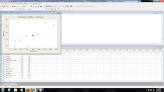 Is it linear? Yes.
Are there any curves? No.
3. Display Descriptive Statistics for each variable of interest
Stats> Basic Stats> Display Descriptive Statistics>

Select Variables of Interest>
 Select OK>
 Analysis of the descriptive statistics informs us that the variable distance is right skewed (mean is greater than the median) while airfare is fairly symmetric.
4. Regression - Gives us a better model for prediction
Stat> Regression> Regression>

Select Variables of Interest>

Select OK>
 We now know that the equation for our regression line is "Airfare = 83.3 + 0.117(Distance)"
83.3 is our y-intercept. Now we have to ask, does it make sense?
Setting X (or distance as in the example) equal to zero, we are left with Airfare = 83.3.
Does this make sense? If you fly zero miles, do you have to pay $83.30? No, it does not make sense in this case. For this line, the y-intercept is irrelevant.
What is the slope of our regression line? 0.117.
What does the slope value tell us? The predicted change in Y for every one unit change in X.
e.g. (The predicted change in airfare for every one mile change in distance)
Using the regression line, by plugging in values for distance.
How much would we expect to pay if we traveled 500 miles?
Airfare = 83.3 + 0.117(500)
Airfare = $141.80, do not round!
Residual = Actual (from original data) - Fit (predicted value from regression line)
Positive residuals - Above the line, underestimate.
Negative residuals - Below the line, overestimate.
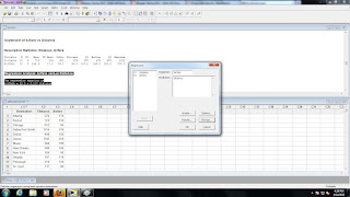


18) Graph> Barchart> Clustered> "Counts of Unique Values>
Correlation coefficient (r): -1 ≤ r ≤ +1 (r can be -1 at least and +1 at most, it's stuck between -1 and 1)
Regression: 
The following examples use the Airfares data set available at Blackboard> In Class> ws3_mintab> WS3_Minitab> Minitab 15 Data> Airfares.MTW
1. Correlation
Stat> Basic Stat> Correlation>

Select variables of interest>

Select OK>

The correlation coefficient is 0.795. This tells us that the relationship between distance and airfare is a strong positive linear association.
2. Scatterplot
Stat> Regression> Regression>

Simple>

Select Variables of Interest>

Select OK>

Are there any curves? No.
3. Display Descriptive Statistics for each variable of interest
Stats> Basic Stats> Display Descriptive Statistics>

Select Variables of Interest>


4. Regression - Gives us a better model for prediction
Stat> Regression> Regression>

Select Variables of Interest>

Select OK>

83.3 is our y-intercept. Now we have to ask, does it make sense?
Setting X (or distance as in the example) equal to zero, we are left with Airfare = 83.3.
Does this make sense? If you fly zero miles, do you have to pay $83.30? No, it does not make sense in this case. For this line, the y-intercept is irrelevant.
What is the slope of our regression line? 0.117.
What does the slope value tell us? The predicted change in Y for every one unit change in X.
e.g. (The predicted change in airfare for every one mile change in distance)
Using the regression line, by plugging in values for distance.
How much would we expect to pay if we traveled 500 miles?
Airfare = 83.3 + 0.117(500)
Airfare = $141.80, do not round!
How much would we expect to pay if we traveled from Baltimore to San Francisco (2815 miles)
Airfare = 83.3 + 0.117(2815)
Airfare = $412.66
This is an example of extrapolation. Extrapolation is going beyond the range of our data to make predictions. Do not do this, it is extremely inaccurate and unreliable. Why is it extrapolation? Our highest observation was around 1500, 2814 is 1314 miles away from this and most of the data that the line is based on is clustered around 500. ("The Lurking Dangers of Extrapolation") The book discusses this on page 191.
5. Residuals - Outliers with respect to the regression
Residual = Actual (from original data) - Fit (predicted value from regression line)
Positive residuals - Above the line, underestimate.
Negative residuals - Below the line, overestimate.
Stat> Regression> Regression>
Select Storage>

Check Residuals and Fits>

Select OK>

Influential Point (Influential Observation) - Dramatically impacts regression equation when removed.
Residual plot - Original x variable plotted on the x-axis and the residuals plotted on the y-axis.
Graph> Scatterplot > With Regression>

Select variables of interest (original x variable on x, residuals on y)>

Select OK>


With a residual plot we are looking for two things with every residual plot.
1) The same number of dots above and below the line (approximately).
2) Random distribution, no obvious pattern.
Only when both of these conditions are met can we claim: "the line does as good as we can do for making predictions"
This video may help clarify any questions you have about regressions thus far.
This video may help clarify any questions you have about regressions thus far.
Subscribe to:
Comments (Atom)