03-14-2012

4.1 #15) Categorical variables require cross-tabulation.
18) Graph> Barchart> Clustered> "Counts of Unique Values>

Correlation coefficient (r): -1 ≤ r ≤ +1 (r can be -1 at least and +1 at most, it's stuck between -1 and 1)

 Regression:

The following examples use the Airfares data set available at Blackboard> In Class> ws3_mintab> WS3_Minitab> Minitab 15 Data> Airfares.MTW 

1. Correlation
Stat> Basic Stat> Correlation> 

Select variables of interest>

Select OK>

 The correlation coefficient is 0.795. This tells us that the relationship between distance and airfare is a strong positive linear association.


2. Scatterplot
Stat> Regression> Regression> 

Simple>

Select Variables of Interest>

Select OK>

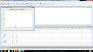
Is it linear? Yes.
Are there any curves? No.

3. Display Descriptive Statistics for each variable of interest
 Stats> Basic Stats> Display Descriptive Statistics> 

Select Variables of Interest>

Select OK>

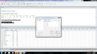
 Analysis of the descriptive statistics informs us that the variable distance is right skewed (mean is greater than the median) while airfare is fairly symmetric.


4. Regression - Gives us a better model for prediction

Stat> Regression> Regression>

Select Variables of Interest>

Select OK>

We now know that the equation for our regression line is "Airfare = 83.3 + 0.117(Distance)"
83.3 is our y-intercept. Now we have to ask, does it make sense?
Setting X (or distance as in the example) equal to zero, we are left with Airfare = 83.3.
Does this make sense? If you fly zero miles, do you have to pay $83.30? No, it does not make sense in this case. For this line, the y-intercept is irrelevant.


What is the slope of our regression line? 0.117.
 What does the slope value tell us? The predicted change in Y for every one unit change in X.
e.g. (The predicted change in airfare for every one mile change in distance)


Using the regression line, by plugging in values for distance.

How much would we expect to pay if we traveled 500 miles? 
Airfare = 83.3 + 0.117(500)
Airfare = $141.80, do not round!

How much would we expect to pay if we traveled from Baltimore to San Francisco (2815 miles)

Airfare = 83.3 + 0.117(2815)

Airfare = $412.66

This is an example of extrapolation. Extrapolation is going beyond the range of our data to make predictions. Do not do this, it is extremely inaccurate and unreliable. Why is it extrapolation? Our highest observation was around 1500, 2814 is 1314 miles away from this and most of the data that the line is based on is clustered around 500. ("The Lurking Dangers of Extrapolation") The book discusses this on page 191.

5. Residuals - Outliers with respect to the regression 

Residual = Actual (from original data) - Fit (predicted value from regression line)
Positive residuals - Above the line, underestimate.
Negative residuals - Below the line, overestimate.

Stat> Regression> Regression>

Select Storage>

Check Residuals and Fits>

Select OK>

Influential Point (Influential Observation) - Dramatically impacts regression equation when removed.

Residual plot - Original x variable plotted on the x-axis and the residuals plotted on the y-axis.

Graph> Scatterplot > With Regression>

Select variables of interest (original x variable on x, residuals on y)>

Select OK>

With a residual plot we are looking for two things with every residual plot.

1) The same number of dots above and below the line (approximately).

2) Random distribution, no obvious pattern.

Only when both of these conditions are met can we claim: "the line does as good as we can do for making predictions"

This video may help clarify any questions you have about regressions thus far.