02-29-2012

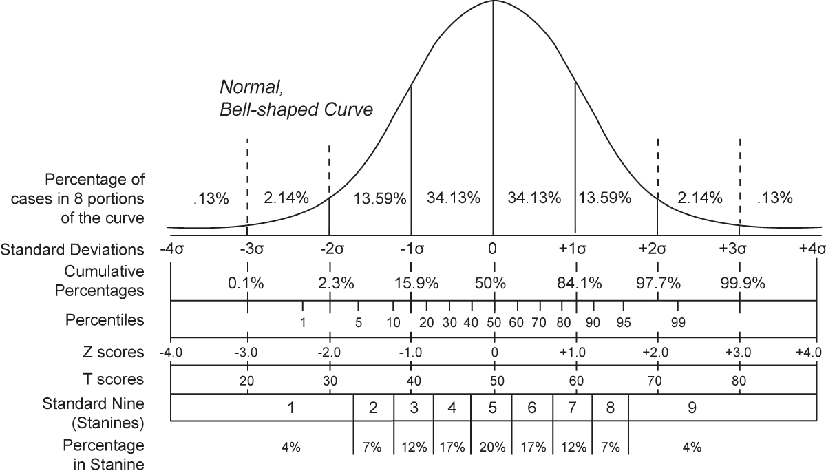
Empirical Rule of Statistics, applies to all standard/normal/symmetrical distributions:
If you travel out to 1 standard deviation, you collect 68% of the observations.
If you travel out to 2 standard deviation, you collect 95% of the observations.
If you travel out to 3 standard deviation, you collect 99.7% of the observations.
Anything beyond 3 standard deviations is unexpected, but we will continue to use the 1.5IQR method to declare outliers.
If  the z-score is exactly average, the value is 0. This is the 50th percentile.

If you are unclear on any of this please watch this video

3.5) Applying the Empirical Rule
6. Normal Distribution, never assume normal. Must be standard!
9. No cannot use it. However if we could, μ =100,  σ = 10, drawing it. we determine that values of 80 and 120 correspond to 2 standard deviations, which would catch 95% of the data.

Example: Birth weights
μ = 3300 grams,  σ = 570 grams

Drawing a Normal Distribution we have a 3300 at the center.
Moving to the right: +1 is 3870, +2 is is 4440, +3 is 5010.
Moving to the left: -1 is 2730, -2 is 2160, -3 is 1590.

Criteria for a "low birth weight" is a weight of less than 2500 grams. Where does this fall on our distribution?
(2500-3300)/570 = 1.4 standard deviations BELOW average.
What is the percentage of observations within one standard deviation? 68%
What is the percentage of observations below one standard deviation? 84% (50% + 34%, why 50%? because we know fifty percent of the data lies on either side of the mean. Why 34%? because we know 68% of the data falls within 1 standard deviation, so if one half of the 68% is already accounted for in the previously mentioned 50% we are left with the other half and half of 68% is 34%.)

How many standard deviations away from the mean is a birth weight of 3600 grams? (3600-3300)/570 = +0.53
How many standard deviations away from the mean is a birth weight of 4536 grams? (4536-3300)/570 = +2.17
How many standard deviations away from the mean is a birth weight of 5443 grams? (5443-3300)/570 = +3.76
Suppose we are given a z-score and want to determine the original observation.
Continuing with our birth weight distribution, we have a z-score of: -3.76 and we want to know the weight that corresponds with this extremely low z-score.
How do we set it up? We just use some algebra on the z-score formula we already know:

So for our example:

-3.76 = (x - 3300)/570
-3.76(570) = x -3300 (multiplying both sides by the standard deviation)
-2143.2 = x - 3300
1156.8=x (adding the mean to both sides)

02-27-2012

3.2 #6) standard deviation. Type numbers into minitab, stat>basic stat>display descriptive statistics.

3.6 #5) Robust Measures = 1.5 IQR.
It's possible, all values between q1 and q2, would have to be equal. It's possible that they're all sevens. The resulting boxplot would just be a line.
c) Mean is larger than q3? when set is heavily skewed right.
d) mean is smaller than q1? when set is heavily skewed left.
e) median smaller than q1? impossible.
f) Q3 cannot be smaller than c1, but can be equal.

3.6 #9) Organize them in descending order, find the median (observations 5 and 6), find q1 (observation 3), find q3 (observation 8).

3.6 #31) 10 calories, 50% of the cereals are within 10 calories of each other.

Quantitative data uses mean and median.
Asterisks in a Minitab produced graph denote an outlier.


3.4 Measures of Position (Z-Scores)
What are the measures of spread? range, IQR, five number summary, standard deviation.
What is the best measure of spread? Standard deviation, tells you the average distance an observation is from the mean.

Percentile - Percentage of the data is below a given number. E.G. 95% of people are below this score, 5% of people are above this score.
Median = 50th percentile.
Q1 = 25th percentile.
Q3 = 75th percentile.
Simply a relative measure of position.

To find the observation corresponding to a percentile:

index = (percentile value/100)number of observations.

Example for 85th percentile of 12 observations: i = (85/100)12
i=10.2. The 85th percentile is found in the 11th box, because if we rounded down to 10 it would not reflect the 85th percentile.


Z-Score - Standardized Measure (score) used to compare unlike distributions.

SAT
Maximum score: 2400
Mean score: 1500
Standard deviation: 150

ACT
Maximum score: 36

Mean score: 24
Standard deviation: 2.5

Bob scored a 1700 on the SAT.
Sandy scored a 27 on the ACT.
Who scored higher? We cannot tell directly since SAT and ACT are measured on different scales. How do we find out? We use Z-scores to determine how many standard deviations away from the mean each person is.
Z-score formula for a parameter from a population:

 Z-score formula for a statistic from a sample:

Z-score value = (observed value - expected value (mean)) /standard deviation

Bob: (1700-1500)/150 = 1.33 standard deviations above the mean.
Sandy: (36-24)/2.5 = 1.2 standard deviations above the mean.
Knowing this, who performed better on the standardized tests? Bob

Example from p. 129.
Mean blood level for lead poisoning: 31.4 micrograms/deciliter
Standard deviation of blood level for lead poisoning: 14.2 micrograms/deciliter

Ryan: 78.26 μg/dl
Megan: 1.58 μg/dl
Kyle: 55.54 μg/dl
Calculate the z-score for each person.
Ryan: 3.3, Megan: -2.1, Kyle: 1.7

If you are unclear on any of this please watch this video

02-22-2012

3.1 # 7B) Put them in order (from least to greatest) then find the middle. If it's even we will take  the two middle observations sum them then divide by two in order to create the median. If it's odd add one to the total number of observations and divide by two to find your median observation.
7C) 15 and 5 are the mode.

#25) Mean, median and mode are all halved

3.2 #26) Don't care about variance. Range = Highest value-lowest value. Std Deviation: Just pull up data sets from publisher's site or CD-ROM and use Minitab (Stat>Basic Stat>Descriptive Statistics)

Standard Deviation - What's normal and acceptable variability (sets the limit for how far is too far)

3.6 Robust Measures
Range is determined by subtracting the lowest value from the highest value, which includes outliers (on either end). It merely measures the distance from top to bottom, doesn't tell you anything in between.

Interquartile Range (IQR) - Contains the middle 50% of the data. It's a much better "range" to give as it excludes outliers.
IQR = Upper Quartile (Q3)- Lower Quartile (Q1).

What's a quartile? It's basically the median of your median. Given median is "the middle" if you find the middle of middle you are given a quarter. You use the same mathematical methodology to find quartiles that you used to determine median.

To get an even better picture of our data set, we will use the Five Number Summary (FNS).
What Five Numbers? (from left to right) Minimum, Q1, Median (Q2), Q3, Maximum.

What is a distribution? Pattern of variability. How does the data change from one observation to another.

1.5IQR - Method of calculating outliers with the IQR. Multiply 1.5 x (IQR value)
Add the (1.5IQR value) to Q3 (Q3 + (1.5IQR value)), any observations greater than this number is considered an outlier.
Subtract the (1.5IQR value) from Q1 (Q1 - (1.5IQR value)), any observations less than this number is considered an outlier.
Exercise comparing average monthly high temperatures for San Francisco, CA and Raleigh, NC.


San Francisco:

58, 59, 61, 62, 64, 65, 65, 68, 68, 69, 70, 71

1. What is the mean (x-bar) temperature? 65
2. What is the median temperature? 65
3. What is the minimum temperature? 58
4. What is the maximum temperature? 71
5. What is the temperature range? 13
6. What is the temperature of the first quartile (Q1)? 61.5
7. What is the temperature of the third quartile (Q3)? 68.5
8. What is the interquartile range (IQR)? 7

Interpretation of the IQR: the middle 50% varies by 7 degrees.

Raleigh:

49, 52, 53, 60, 61, 70, 71, 78, 80, 84, 86, 88

1. What is the mean (x-bar) temperature? 69.3
2. What is the median temperature? 70.5
3. What is the minimum temperature? 49
4. What is the maximum temperature? 88
5. What is the temperature range? 39
6. What is the temperature of the first quartile (Q1)? 56.5
7. What is the temperature of the third quartile (Q3)? 82
8. What is the interquartile range (IQR)? 25.5

Interpretation of the IQR: The middle 50% varies by 25.5 degrees.

Given what you now know about the climate of these two cities, which city would you expect has a larger standard deviation? Which city would you expect has a smaller standard deviation? San Francisco will have a smaller standard deviation because it has lower total variability.
Minitab exercises
Getting the Five Number Summary from Minitab


Get the temperature data set off Blackboard> Course Documents>"Temps"
Stat> Basic Stats> Display Descriptive Statistics>

Select the variables of interest (both "San Francisco" and "Raleigh").

Then select "OK" (highlighted text contains five number summary)

Interpreting the data: "Most of the time it will be between 61 and 69 degrees in San Francisco"



How to construct a Boxplot in Minitab
Graph> Boxplot>

Select "Multiple Y's - Simple"

Select the variables of interest (both "San Francisco" and "Raleigh").

Select "OK"

Interpretation: Line connects minimum to Q1 and Q3 to maximum. Box contains IQR (Q1 to Q3) with middle 50% of the data.

Constructing a Boxplot in Minitab pt. II
Blackboard> Course Documents > Golf PGA '09

Create a new variable to make the data easier to manage.
Calc> Calculator

Store result in a new column to not overwrite any data, expression is Earnings divided by 1,000,000.

Select "OK" (output is highlighted)

Stat> Basic Stat> Display Descriptive Statistics>

Select the new column (e.g. "earnings in millions")

Select "OK"

Graph > Boxplot

Select "One Y - Simple"

Select variable of interest (e.g. "earnings in millions"), then select "Scale"

After you've selected "Scale", check "Transpose value and category scales"

Select "OK" to produce the boxplot

Notice that this boxplot is horizontal? That's the result of "Transpose value and category scales". Graph is right-skewed.
Note: Minitab produces modified boxplots, meaning that it goes to the value nearest the 1.5 IQR that doesn't exceed that 1.5 IQR value. Asterisks indicate outliers.

02-15-2012

Median is resistant to outliers (not greatly influenced by outliers)
Mean is not resistant to outliers, prone to follow the tail (at the mercy of outliers)

In class exercise with mean and median using height of class members.
Mean was 66.9 inches
Median was 66 inches

Measures of Variability (Spread)

Range - "Mostly useless, can be beneficial on occasion" To find the range you subtract the highest value of your data set from the lowest value of your data set. Using our class height as an example the tallest member is 78 inches, while the shortest individual is 60 inches. 78 - 60 = 18 inches.

Variance - Not interested in this measure of variability, skip any homework questions asking for variance.

Standard Deviation - "Think of it as the average difference from the mean or the 'acceptable deviation'."

Standard deviation for a parameter:

• σ = Standard Deviation of parameter from a population
• N = Population size
• xi = Individual observation
• μ = Mean of the parameter from a population

Standard Deviation for a statistic:

• s = Standard Deviation of statistic from a sample
• n = Sample size
• xi = Individual observation 
• x-bar = Mean of the statistic from the sample

As complicated as these expressions look they are basically saying: "Sum the squares of all the individual observations (observed value) -  mean (expected value), divide this number by the sample size less one (or the population size), then take the square root of that number. The resulting number is your Standard Deviation.
 

• You cannot know the standard deviation without knowing the following: mean, sample size, individual values.

Going back to the class height data, the standard deviation in height is 3.821 inches. So if you were to grab someone from our class at random you would not be surprised if their height was between 63.1 inches and 70.7 inches.

Using Quiz 1 test results:

• μ = 67%
• Median = 73%
• σ = 23.87%
• range = 100

Describe this distribution.

The mean  is smaller than the median, therefore skewed left.

However, this data is not reflective of the class. Notice that the range is 100, the data set is accounting for people who have not taken the quiz yet (people with zeroes).

Taking this into account and adjusting the data set accordingly:

• μ = 70.5%
• Median = 76.7%
• σ = 18.58%
• range = 67 (from 100-33)

Notice that the Mean has shifted upward because it is no longer being weighed down by the zeroes.
This change in mean also alters the standard deviation because the mean is used to calculate the standard deviation.
If you are unclear on any of this please watch this video 

02-13-2012

Measures of center:

Mean (the arithmetic mean or average) - Add all observations up and divide by the number of observations. Good for quantitative variables. Easily influenced by outliers.

• If the mean is with respect to a population we use: μ (mu)
• If the mean is with respect to a sample we use: x̅ (x bar)

X bar = the sum (sigma) of numbers from i (which equals 1 in this case) to n (number of observations) all divided by n (number of observations). As complex as this expression looks, it's really shorthand for: (observation1 + observation2 + observation3 + observation4 + observation5) / 5. Why 5? Because there are 5 observations

Median (middle) - Value exactly in the middle of the data after the data is put in order (ascending or descending). Good for quantitative variables.
Calculating median for odd numbers: (n+1)/2
Calculating median for even numbers: (middle 2 observations)/2

Mode - Most frequent number/observation. Good for quantitative and categorical variables, but usually used for categorical variables.

If you are unclear on any of this please watch this video

Minitab exercises:

File from Blackboard > Course Documents > Golf > "PGA Earnings 09.mtw"

Stat > Basic Stats

Stats > Basic Stats > Display Descriptive Statistics

Select "Earnings"

Click "OK" which will yield these descriptive statistics:

 Please make note of the Mean and Median, then make a histogram (if you forgot how check 02-06-2012) to check for outliers.

Notice that outlier? Let's see what our Mean and Median would look like without Tiger Woods. Replace his "Earnings" with an asterisk (*) this tells Minitab to skip this observation.

Run the Descriptive Statistics again, make a note of Mean and Median.

What would happen to the Mean and Median if we made the outlier even more drastic? Add an extra zero to Tiger Woods' earnings.

Run the Descriptive Statistics on last time, note the Mean and Median.

What have we learned?
"The mean is more susceptible to outliers because everyone is include in the mean value"
If the data is skewed: use the median.
If the data is symmetric: use the mean.

However, we will always be use both (mean and median).

QUIZ #1!

Quiz #1 is today (2/13/2012)

"DON'T FORGET to bring a Blue Book."

Freaking out?

Don't freak out! If you have any last minute questions feel free to stop by the SJC LRC and ask, I plan to be in there from 11:00-12:20 studying.  Best of luck on your first quiz!

02-08-12

2.1) #15. Assume 6000, multiply percent by 6000 to find counts. Barchart for categorical data from Table.

41. Supermarkets - 73357/198514 = 36.94% (37%)
Delicatessens - 6123 / 198514 = 3.1%
SKIP 16! Pie charts are unimportant.

What is a histogram good for? Quantitative Data
How is a histogram different from a bar chart? Data is continuous.

Reviewed Sorting and Calc features of Minitab (02-06-2012)

Exercise: Make a histogram with fit of the "calories/gram" column you created and evaluate the distribution. Is it symmetric? Is it skewed? Where does the center lie? What is the spread? Are there any outliers?

Quiz #1 will cover homework sections assigned up to 2.2
~5 (involved) questions, similar to the "applying concepts" type questions in the textbook.
Everything on the quiz has been covered in class. There are no "trick" questions, take the questions at face value. If you have a question, be safe, ask.
You will need: A blue/green book, which you can purchase in the book store or cafeteria.
You are allowed: a 3x5" card with hand written notes for when you blank

Review questions:
1.  Suppose that the observational units in a study are patients arriving at an emergency room on a particular day.  For each of the following, indicate whether it is a legitimate variable or not.  If it is a variable, classify it as quantitative, binary categorical, or categorical (non-binary).  If it is not a variable, explain why not.
a) blood type
b) whether or not men have to wait longer than women
c) number of patients that arrive before noon
d) number of stitches required

2.  Suppose that you are given a sample of 25 Reese's Pieces candies and asked to record the color of each candy.
(a)  What are the observational units here?
(b) What is the variable here?  Is it categorical (binary?) or quantitative?
(c) Now suppose that each of your classmates is also given a sample of 25 Reese's pieces candies.  Also suppose that everyone is asked to report the percentage of yellow candies in her sample of 25 candies.  Now what are the observational units?  (Be careful -- the observational units are not the same here as they were in part (a).)
(d) Now what is the variable?  Is it categorical (binary?) or quantitative?

3. Researchers at Stanford University studied whether or not reducing children's television viewing might help to prevent obesity. Third and Fourth grade students at two public elementary schools in San Jose were the subjects. One of the schools incorporated a curriculum designed to reduce watching television and playing video games while the other school made no changes to its curriculum. At the beginning and each of the study a variety of variables were measured on each child. These included body mass index, tricep skinfold thickness, waist circumference, waist-to-hip ratio, weekly time spent watching television and weekly time spent playing video games.
a) Identify the type of study
b) Identify the observational units
c) Identify the variables (quantitative or categorical, if categorical are they binary?)

02-06-2012

1.2 # 24) Quantitative, it's a count.
1.3 # 18) Observational - Nothing was imposed, just observing. Predictor: Large families. Response: Church attendance.
19) Observational (no randomization, no control). Predictor: Large bonus, Response: stock prices.
21) "Because it's random"
28c) Predictor: Medication. Response: LDL Levels. Experiment: Trying to prove "cause and effect" of the medication. Treatment: Medication. Control: Placebo.
2.1 #14) Surveying from a website creates bias against individuals without internet access.

What is a frequency? A count.
What is relative frequency? A percent
The graphs of the two are identical other than the Y-Axis.

Reviewed how to use Minitab to create bar charts for both types of frequency (latter half of 2-1-12)

When asked to "interpret data" state the obvious, don't talk about anything beyond what the data shows. (e.g. 18.9% of the people in the class like sports and 8 people listed music as an interest)

• Data sets from the book are available at http://www.whfreeman.com/discostat  under student resources "Data Sets", select Minitab (or whatever software you are planning to use). EX refers to example and TA refers to table.

2.2
No longer interested in categorical, now we are looking at quantitative

Reviewed how to use Minitab to create bar charts for both types of frequency (latter half of 2-1-12)


Histograms - typically report frequency; Each bar represents a range, no gap between items because the data is continuous.
Class width - same on all histograms.
Cut point - always fall to the right.

How to make a Histogram in Minitab:

Graph> Histogram

Graph>Histogram> Simple

Select Age

This histogram results

To modify the classes, double click a bar

Select "Binning" tab

Select "Cut Points"

Select OK, observe the difference.

Double click a bar to modify the graph again, returning to the binning tab.Change the number of intervals, to those desired (3 in this case).

Select OK, observe the difference.

Not happy? Double click a bar to edit.

Change the Midpoint/Cutpoint positions as desired (0 4 7 10, in this case)

Observe the difference. This arrangement of the data shows the majority of child abductions occur between the ages of 4 and 7.

Distribution - Pattern of variablity

1. Types of Distribution
1. Symmetric - Same on both sides. Commonly referred to as the Bell Curve or Standard Normal Distribution.
2. Right skewed - Data is clustered on the left side, tail is on the right.
3. Left skewed - Data is clustered on the right side, tail is on the left.
2. Center - Center of the data not the center of the axis.
3. Spread - Variability, how spread out the data is. Is it clustered tightly together or is it spread out? Currently only interested in the highest and lowest values.
4. Outliers - Way different from everybody else (usually a gap between core of the data and an outlier)

How to Sort data within Minitab:

Data>Sort>

Yields this menu

Select the variables you are interested in sorting (Note: Select the variable you wish to sort by first, then the variable you wish to be sorted. In this example 'Calories' are being sorted with respect to 'Food'.)

Before you click OK, you want to modify where this data is exported. NEVER USE "ORIGINAL COLUMN(S)"! Select "Column(s) of current worksheet" at the bottom of the menu and select a few columns far away from your source data so you don't accidentally overwrite anything!

The highlighted columns on the far right are the result of this sorting

That's all well and good, but who eats an entire carrot cake in one sitting? Perhaps we're better off sorting this data set by calories per gram. What's that? There's no calories per gram column? Look's like we'll just have to make one!

Calc> Calculator

Since we are interested in Calories PER Gram. "Per" denotes division, so let's set up an equation for what we are interested in. Note: Store your result in a column away from your source data to prevent any overwrite accidents.

Now that you have "Calories/Gram", it would be a good idea to sort this new column the way you sorted "Calories" originally so you can know the relationship between the values and the corresponding food item.